• Skip to main content
itrc_logo

Geospatial Analysis for Optimization at Environmental Sites

Home
About ITRC
Navigating this Website
Overview
Fact Sheets
Fact Sheets Overview
Fact Sheet 1: Do You Need Geospatial Analysis?
Fact Sheet 2: Are Conditions Suitable for Geospatial Analysis?
Fact Sheet 3: How is Geospatial Analysis Applied?
Fact Sheet 4: What Software is Available to Help?
PM's Tool Box
PM's Tool Box Overview
Review Checklist
Choosing Methods
Common Misapplications
Optimization Questions
Geospatial Analysis Support for Optimization Questions in the Project Life Cycle
Data Requirements
General Considerations
Methods for Optimization
Geospatial Methods for Optimization Questions in the Project Life Cycle Stages
Release Detection
Site Characterization
Remediation
Monitoring
Closure
Documenting Results
Fundamental Concepts
Fundamental Concepts for Geospatial Analysis
Basic Data Concepts for Geospatial Analysis
Interpolation Methods and Model Prediction
Uncertainty in Geospatial Analyses
Characteristics of Interpolation Methods
Work Flow
Work Flow for Conducting Geospatial Analysis
Geospatial Analysis Work Flow Overview
Perform Exploratory Data Analysis
Select Geospatial Method
Build Geospatial Model
Evaluate Geospatial Method Accuracy
Generate Geospatial Analysis Results
Using Results
Using Analysis Results for Optimization
Plume Intensity and Extent
Trend Maps
Estimating Quantities
Hot Spot Detection
Sample Spacing
Estimating Concentrations Based on Proxy Data
Background Estimation
Quantifying Uncertainty
Remedial Action Optimization
Monitoring Program Optimization
Examples
Examples Overview
Example 1
Example 2
Example 3
Example 4
Methods
Methods Overview
Simple Geospatial Methods
More Complex Geospatial Methods
Advanced Methods
Index of Methods
Software
Software Overview
Software Comparison Tables
Software Descriptions
Workshops and Short Courses
Case Studies
Case Studies Overview
Superfund Site Monitoring Optimization (MAROS)
PAH Contamination in Sediments—Uncertainty Analysis (Isatis)
Optimization of Long-Term Monitoring at Former Nebraska Ordnance Plant (GTS; Summit Envirosolutions)
Optimization of Lead-Contaminated Soil Remediation at a Former Lead Smelter (EVS/MVS)
Extent of Radiological Contamination in Soil at Four Sites near the Fukushima Daiichi Power Plant, Japan (ArcGIS)
Optimization of Groundwater Monitoring at a Research Facility in New Jersey (GWSDAT)
Optimization of Sediment Sampling at a Tidally Influenced Site (ArcGIS)
Stringfellow Superfund Site Monitoring Optimization (MAROS)
Lead Contamination in Soil (ArcGIS)
Stakeholder Perspectives
Additional Information
Project Life Cycle Stages
History of Remedial Process Optimization
Additional Resources
Acronyms
Glossary
Index of Methods
Acknowledgments
Team Contacts
Document Feedback


Geospatial Analysis for Optimization at Environmental Sites
HOME

Uncertainty in Geospatial Analyses

The collection and analysis of environmental data, as well as site management decisions made based on these data, are subject to uncertainty. The most obvious source of uncertainty in geospatial analysis results from the inability to sample everywhere, which means that a range of potential values exist at unsampled locations. Geospatial methods differ in their ability to provide quantitative measures of uncertainty for predictions at unsampled locations. This section provides an overview of the sources of uncertainty resulting from sampling bias and error and from differences in analytical precision. Information about uncertainty from the use of different geospatial methods is presented in Evaluate Geospatial Method Accuracy. The sources of uncertainty should be identified and documented; to the extent possible, the effects of uncertainty should be minimized.

▼Read more

Uncertainty also arises from errors in data collection and modeling, with error being defined as the difference between a true value in nature and a measured or predicted value (Krivoruchko 2011). Specific examples of error contributing to uncertainty in the distribution of a parameter of interest include:

  • Sampling bias and error can result from the collection of samples that are not representative of the spatial and temporal heterogeneity (the underlying variation) of the media being sampled.
  • Locational error can result from imprecise measurement of sample collection locations, which is more or less significant at different study scales.
  • Error in laboratory or field-based analytical techniques can result from using instruments with different precision. This type of error includes error caused by variation that is below the detection capability of the sampling program.
  • Error can be introduced by interpolation methods themselves, which may be caused by using assumptions that are not supported by the data, or by characteristics of the interpolation algorithm such as the tendency of kriging to smooth out spatial variation. The latter example is a form of conditional bias that overestimates small values and underestimates large values (Goovaerts 1997). Interpolation method performance can be evaluated through cross-validation, which compares interpolated to measured values to quantify prediction accuracy.

More complex and advanced geospatial methods recognize that there is error in spatial predictions, and attempt to quantify the resulting uncertainty. At its most basic level, kriging incorporates uncertainty through use of a nugget representing the white noise variation in the model (sampling error, analytical error, or smaller-scale variation that is below the detection of the current sampling program). Kriging also provides prediction standard error estimates that can be used to build a variance map to evaluate uncertainty. Indicator kriging is another way to evaluate uncertainty by generating maps that depict the probability of exceeding threshold values.

Kriging and certain more complex methods of evaluating uncertainty are inherently limited because they focus on local uncertainty associated with single estimate locations and because of the smoothing tendency of kriging. Conditional simulation attempts to better quantify true uncertainty by reconstructing the spatial heterogeneity, or variation, intrinsic to the environmental system investigated. As a result, simulation better assesses spatial uncertainty as whole, or the joint uncertainty considering multiple locations taken together. This method is especially useful for data sets with extreme values and heterogeneity, which is often the case with contaminant concentration data (Goovaerts 1997); see the example of using conditional simulation to create statistical and probability maps for uncertainty analysis.

Sampling Bias and Error

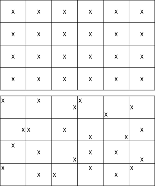
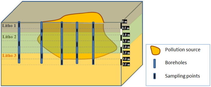
The quality of the results of any geospatial method depends on the quality of the input data. Often, only one sample is collected at each borehole and geological layer, which may introduce bias since the collected sample is assumed to be representative of the entire stratigraphic unit that is being characterized. When sampling for lateral delineation, systematic grid-based sampling may be used for the initial site characterization. This type of sampling, however, may include some bias. Figure 11 includes an example of results from systematic grid-based sampling.

gro_fig_3_5

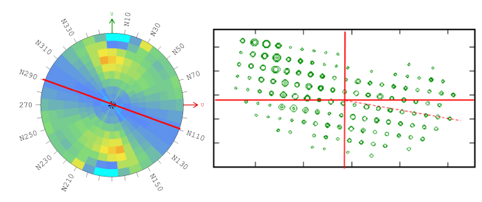
Figure 11. Example of systematic sampling on a 25mx25m grid (left) and possible anisotropy detected along the sampling direction (right). True anisotropy or sampling effect?

▼Read more

Stratified random sampling can be a good alternative to avoid such biases. This approach provides information about different spaced samples, which may improve the knowledge of the experimental variogram. Moreover, this strategy allows some flexibility to resolve the access issues when planning the field investigation. Figure 12 includes examples of systematic sampling and stratified random sampling.

gro_fig_3_6_500_wide

Figure 12. Example of systematic sampling (top) and stratified random sampling (bottom).

If the goal is to identify potential contamination sources, a sampling approach using a cross or a spiral sampling geometry can be implemented. Conducting a sampling strategy by drilling closely spaced boreholes improves the understanding of the contamination and provides better data for fitting the empirical variogram. Figure 13 includes an example of sampling using a cross geometry approach with sampling locations at the grid crossings (sampling points S1, S2, S3, S15, S17, S19 and S20) so that there are more closely spaced sampling locations.

gro_fig_3_7

Figure 13. Example of sampling by using a cross geometry approach near a contamination source.

When sampling for vertical delineation, collecting samples from each geological unit is a good approach. It is important to collect samples at different depths in the same geological layer (see Figure 14). This approach provides information about the attenuation of the contamination at depth.

gro_fig_3_8

Figure 14. Example of vertical sampling near a contamination source on a site consisting of three different geological units.

Often, the delineation of the contamination is less complete in the vertical direction than in the horizontal direction. Using field-based measurement technologies (for example, mobile lab) during the initial characterization step facilitates the complete delineation of contaminant sources (USEPA 2003; ITRC 2003; and ITRC 2007). These methods can reduce uncertainties.

Additional information can be found in the USEPA (2002a) guidance on choosing a sampling design, and the ITRC (2012a) guidance on incremental sampling methodology.

Analytical Precision

Uncertainty is present in the analytical results obtained from laboratories and should be clearly identified. Similarly, if field-based measurement technologies are used, the accuracy of each device must be identified. In addition, the analysis carried out in the laboratory is based on a small fraction of the total sample collected, which is a minimal part of the geological unit being characterized. This result is then assumed to be representative of the whole geological unit. This bias should be taken into account when interpreting the final results.

▼Read more

Which analytical results to include in the geospatial modeling should be considered when planning the evaluation. For example, what samples should be included as representative for a contamination source? Samples with concentrations slightly below a remediation threshold may or may not be considered part of the contamination source based on their physical location adjacent to higher concentration results. Also, decisions about concentration results that are below a laboratory detection limit should be considered. More information about managing nondetect data in statistical analyses is included in GSMC-1, Section 5.7.

These and other sources of uncertainty are difficult to manage. The strategy for managing sources of uncertainty for a specific project should be documented so that the geospatial modeling results are more transparent and the impacts of the uncertainties can be minimized.

USEPA offers additional guidance on this topic (USEPA 2006a; USEPA 2006b; USEPA 2008; USEPA 2011a).

image_pdfPrint this page/section


GRO

web document
glossaryGRO Glossary
referencesGRO References
acronymsGRO Acronyms
ITRC
Contact Us
About ITRC
Visit ITRC
social media iconsClick here to visit ITRC on FacebookClick here to visit ITRC on TwitterClick here to visit ITRC on LinkedInITRC on Social Media
about_itrc
Permission is granted to refer to or quote from this publication with the customary acknowledgment of the source (see suggested citation and disclaimer). This web site is owned by ITRC • 1250 H Street, NW • Suite 850 • Washington, DC 20005 • (202) 266-4933 • Email: [email protected] • Terms of Service, Privacy Policy, and Usage Policy ITRC is sponsored by the Environmental Council of the States.