Example 3
| Example 3: Co-kriging and Validation |
|---|
|
Application: Sampling optimization, site characterization, contaminant fate and transport, remediation progress prediction
Application Summary: Co-kriging is a multivariate geostatistical method used to integrate different data sources that are sampled at varying sampling densities, spatial resolutions, or purposes. Often, co-kriging alleviates data gaps by fusing spatially dense proxy sample data with other sparse direct sample data to generate predictions. Proxy data are good surrogates to other direct measurements if they correlate with the primary measurements. Certain proxy data can be generated from field instrument measurements, which are relatively cheaper, quicker and less invasive compared to direct sampling. In this case, co-kriging was used to predict soil moisture content in unsampled locations using geophysics and soil coring data. Soil moisture influences the fate and distribution of dissolved contaminants, which is difficult to predict in unsaturated soils that are not at steady state. Geophysical measurements, such as bulk electrical conductivity, are sensitive to soil moisture and other conductive soil properties. As such, they are a good proxy data measurement to estimate soil moisture with increased spatial continuity and finer spatial resolution. Software: Isatis Methods: EDA, cross-variography, ordinary co-kriging Data Requirements: Proxy data spatially correlate with other direct sampling measurements. Case specific. Reference: Chilès and Delfiner 1999; Ecole Des Mines De Paris 2013; Landrum 2013 |
|
Approach: Real-time, on-the-go bulk surface electrical conductivity measurements were collected in tandem with primary soil moisture measurements. There were approximately 10,000 electrical conductivity data points over 40-acre landscape, that were collected in less than 4 hours using field equipment. The sampling resolution ratio between the field equipment measurement and direct soil sampling was approximately 100:1.
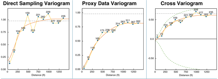
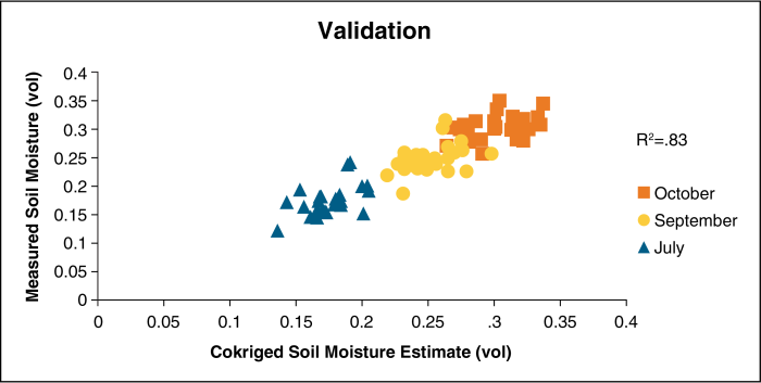
For each sampling date, an independent subset of soil moisture samples (validation subset) was collected to verify the accuracy of the co-kriged estimates. This sample subset was not used to generate co-kriged estimates. The validation samples were collected simultaneously with samples used for model calibration. It was important to collect the validation samples simultaneously because soil moisture content is highly variable over time, depending on the time of day and recent rainfall activity. The number of validation samples was about 20% of the total number of soil samples collected to perform co-kriging. The validation sample locations were randomly selected across the area investigated. Ordinary co-kriging was used to generate soil moisture spatial estimates. Exploratory data analysis was performed to assess for spatial outliers, stationarity and shared spatial autocorrelation between the two measurements (Figure 55). The conductivity data and direct soil moisture measurements were standardized using Gaussian anamorphosis. Variogram modeling was then performed. Cross-validation statistics were used to choose the best fit model to subsequently perform co-kriging. Ordinary block co-kriging was used to generate spatial estimates of soil moisture for each sampling date. Validation was performed to assess the accuracy of spatial estimates. Results: Cross-validation statistics show that the fitted cross-variogram model was adequate for generating spatial estimates. Validation showed that spatial estimates were accurate (Figure 56). Co-kriged results illustrate greater spatial detail in comparison to kriging direct soil moisture data due to higher data density. This detail can lend better insight into preferential flow pathways and localize areas of potential concern with regards to the fate and transport of soil contaminants. |
| Cross-Validation Statistics | ME | VE | MSE | VSE | R2 |
|---|---|---|---|---|---|
| July Soil Moisture | 3.2 x 10⁻² | 0.43 | -3.1 x 10⁻² | 0.69 | 0.75 |
| September Soil Moisture | 1.2 x 10⁻³ | 0.55 | -3.7 x 10⁻³ | 0.91 | 0.67 |
| October Soil Moisture | -5.1 x 10⁻² | 0.51 | -4.9 x 10⁻² | 0.83 | 0.69 |
| Notes: Cross-validation statistics generate the statistical metrics using the same sample data used to generate the estimates. (ME) Mean error – measure the degree of estimate unbiasedness and should be close to zero. (VE) Variance of error – measures precision of estimates and should be as small as possible. (MSE) Mean standardized error – measure the degree of estimate unbiasedness and should be close to zero. (VSE) Variance of the standardized error – ratio of the kriging variance to the sampled variance and should be close to 1. R2 – correlation between the modeled estimates and true values should be close to 1. |
|||||
Figure 55. Variogram models fitted to the direct and proxy sampled data. The cross-variogram is used to optimize the search neighborhood for generating co-kriging estimates.
Source: Landrum 2013.
| Validation Statistics | ME | MSE | VSE |
|---|---|---|---|
| July | 1.6 x 10⁻⁴ | 9.1 x 10⁻³ | 1.7 |
| September | 3.9 x 10⁻³ | 0.21 | 1.81 |
| October | -3.5 x 10⁻³ | -0.17 | 1.7 |
| Notes: Validation Statistics generate an unbiased assessment of prediction accuracy and precision by comparing the predictions to an independent validation sample data set rather than the data set used to generate the predictions. (ME) Mean Error – close to zero indicating the estimates are unbiased. (VSE) Variance of Standardized Error – slightly above 1 for all three sampling dates, but are within the tolerance threshold (Chilès and Delfiner 1999), due to the small number of validation samples. |
|||
Figure 56. Scatterplot of measured soil moisture content (validation sample set) versus co-kriged soil moisture estimates.
Source: Landrum 2013.

