• Skip to main content
itrc_logo

Geospatial Analysis for Optimization at Environmental Sites

Home
About ITRC
Navigating this Website
Overview
Fact Sheets
Fact Sheets Overview
Fact Sheet 1: Do You Need Geospatial Analysis?
Fact Sheet 2: Are Conditions Suitable for Geospatial Analysis?
Fact Sheet 3: How is Geospatial Analysis Applied?
Fact Sheet 4: What Software is Available to Help?
PM's Tool Box
PM's Tool Box Overview
Review Checklist
Choosing Methods
Common Misapplications
Optimization Questions
Geospatial Analysis Support for Optimization Questions in the Project Life Cycle
Data Requirements
General Considerations
Methods for Optimization
Geospatial Methods for Optimization Questions in the Project Life Cycle Stages
Release Detection
Site Characterization
Remediation
Monitoring
Closure
Documenting Results
Fundamental Concepts
Fundamental Concepts for Geospatial Analysis
Basic Data Concepts for Geospatial Analysis
Interpolation Methods and Model Prediction
Uncertainty in Geospatial Analyses
Characteristics of Interpolation Methods
Work Flow
Work Flow for Conducting Geospatial Analysis
Geospatial Analysis Work Flow Overview
Perform Exploratory Data Analysis
Select Geospatial Method
Build Geospatial Model
Evaluate Geospatial Method Accuracy
Generate Geospatial Analysis Results
Using Results
Using Analysis Results for Optimization
Plume Intensity and Extent
Trend Maps
Estimating Quantities
Hot Spot Detection
Sample Spacing
Estimating Concentrations Based on Proxy Data
Background Estimation
Quantifying Uncertainty
Remedial Action Optimization
Monitoring Program Optimization
Examples
Examples Overview
Example 1
Example 2
Example 3
Example 4
Methods
Methods Overview
Simple Geospatial Methods
More Complex Geospatial Methods
Advanced Methods
Index of Methods
Software
Software Overview
Software Comparison Tables
Software Descriptions
Workshops and Short Courses
Case Studies
Case Studies Overview
Superfund Site Monitoring Optimization (MAROS)
PAH Contamination in Sediments—Uncertainty Analysis (Isatis)
Optimization of Long-Term Monitoring at Former Nebraska Ordnance Plant (GTS; Summit Envirosolutions)
Optimization of Lead-Contaminated Soil Remediation at a Former Lead Smelter (EVS/MVS)
Extent of Radiological Contamination in Soil at Four Sites near the Fukushima Daiichi Power Plant, Japan (ArcGIS)
Optimization of Groundwater Monitoring at a Research Facility in New Jersey (GWSDAT)
Optimization of Sediment Sampling at a Tidally Influenced Site (ArcGIS)
Stringfellow Superfund Site Monitoring Optimization (MAROS)
Lead Contamination in Soil (ArcGIS)
Stakeholder Perspectives
Additional Information
Project Life Cycle Stages
History of Remedial Process Optimization
Additional Resources
Acronyms
Glossary
Index of Methods
Acknowledgments
Team Contacts
Document Feedback


Geospatial Analysis for Optimization at Environmental Sites
HOME

Simple Geospatial Methods

Simple geospatial methods estimate values at unsampled points with no statistical error model. They work best with larger data sets. No statistical assumptions are required, so they can be a quick, simple approach to modeling spatial trends. These methods, however, do not quantify prediction uncertainty. This section presents typical uses for simple geospatial methods, such as inverse distance weighting, Voronoi diagrams/Thiessen polygons, and natural neighbor interpolation. The assumptions, strengths, and weaknesses of each method are described, as well as guidance on using the method results.

Inverse Distance Weighting

Inverse distance weighting (IDW) interpolation applies multiplier values to the data points during interpolation so that the influence of one data point relative to another decreases with distance (d), using the weighting function w(d) = 1/dp, where the exponent “p” (or sometimes called weighting power) is usually user-specified. Higher exponent values make points far from a grid node have less effect on the interpolation at that grid node. As the exponent increases, there is less averaging, and the grid node value approaches the value of the nearest data point. As the exponent decreases, there is more averaging, and the weights are more evenly distributed among the surrounding data points (Golden Software 2002). This method is usually available in computer interpolation programs because it is fast, simple, and can accommodate very large data sets.

IDW normally behaves as an exact interpolator, with predicted values exactly coinciding to data values at measurement locations. Because there is no theoretical basis for selecting parameters, the power and search neighborhood terms should be specified based on minimizing cross-validation error. One characteristic of IDW interpolation is the generation of contour maps with bull’s-eye patterns around data points. Some software programs enable smoothing of contours, but this practice may not eliminate the bull’s-eye effect.

Typical Applications

▼Read more

Interpolating spatial data to create contour maps and grids used in surface and volume calculations.

Using this Method

▼Read more

IDW is best suited as an interpolation method for large data sets collected at a high (spatial) density; for example, a refined sampling grid. A lower exponent value (weighting power) will generally create a smoother, more averaged surface. Using an exponent less than 1 should be avoided because it can cause data points far away from prediction locations to influence predictions more than those that are close, contradicting the main rationale for the interpolation (Krivoruchko 2011).

Assumptions

▼Read more

The main assumption of IDW is that data values that are closer to each other are more similar than those that are further away.

Strengths and Weaknesses

▼Read more

The strengths of this method are:

  • IDW efficiently interpolates very large data sets.
  • IDW is simple to understand and implement in many different computer programs.

The weaknesses of this method are:

    • IDW often produces contours with bull’s-eyes representing mounds or depressions in the surface that have no conceptual explanation. This result is due to a scarcity of samples around a data point that differs appreciably from neighboring samples.
    • IDW does not produce good results when used to contour smaller data sets, especially those representing smoothly transitioning properties such as groundwater elevations.
    • IDW interpolation is not based on the spatial correlation of the data set and cannot estimate uncertainty of the interpolated values at unsampled locations. Cross-validation can be used to evaluate the model’s depiction of measured values.

Understanding the Results

▼Read more

Results of IDW interpolation should be compared to the CSM to evaluate whether there are any valid explanations for bull’s-eyes in the surface (for example, pumping or injection wells). The accuracy of IDW interpolation can be assessed and compared to other methods through cross-validation, validation, and field verification.

In the context of optimization, see how to use the results of the geospatial methods to address specific optimization questions.

Further Information

▼Read more

The case study describing optimization of the remediation of lead contaminated soil at a former lead smelter uses IDW interpolation.

Additionally, see guidance on IDW interpolation in Surfer, ArcGIS, and other computer contouring software.

Thiessen Polygons, Delaunay Triangulation Diagrams and Voronoi Diagrams

Two closely related methods of characterizing spatial distribution and influence of sample points are Thiessen polygons and Delaunay triangulations. In each of these methods, the sampling area is divided into regions containing one sampling point. The regions then can be weighted according to the size of the area relative to the total area. For example, concentrations at unsampled points are estimated using a weighted average of the concentrations of adjacent points using the polygon areas for the weights.

▼Read more

Given a set of points [P1, P2, … PN], Voronoi diagrams are used to divide space into regions, so that each region contains one point Pj and each point within the region is closer to Pj than to any other point Pk where k ≠ j. These regions are called Voronoi cells or Thiessen polygons. Figure 58A is an example of a space divided according to Voronoi diagrams, in which each colored polygon is a Voronoi cell, each containing one dot, where the dots represent the points [P1, P2, … PN]. Note that every point within a given polygon is closer to the dot in its own polygon than to any other dot.

Voronoi diagrams are generated from a Delaunay triangulation. In two dimensions, a Delaunay triangulation connects a set of points [P1, P2, … PN] to form triangles, so that no point Pj is in the interior of the circumcircle of any triangle. Figure 58B shows the Delaunay triangulation used to generate the Voronoi cells of Figure 58A. In Figure 58B, the points [P1, P2, … PN] are located at the vertices of the triangles.

gro_fig_8_1_larger_dots

Figure 58. A) (Left) A series of points, indicated by dots, in two dimensions with the space divided into Voronoi cells (or Thiessen polygons), represented as colored polygons; B) (Right) The Delaunay triangulation used to generate the Voronoi cells in A. The same points, represented as dots in A), are the vertices of the triangles in B).
Source: Images generated using the algorithm of Paul Chew (Chew 2007), Cornell University.

The perpendicular bisectors of the Delaunay triangles form the edges of the Voronoi polygons. Figure 59 shows the Delaunay triangulation and the Voronoi diagrams for a set of points. Delaunay triangles are shown in heavy lines. The lighter lines are the edges of the Voronoi polygons. Note that the edges of the Voronoi polygons bisect the edges of the Delaunay triangles. In three dimensions, a Delaunay triangulation forms tetrahedra. Sometimes the Voronoi cells/Delaunay triangles are referred to as Voronoi/Delaunay mesh.

gro_fig_8_2

Figure 59. A set of points shown as vertices of Delaunay triangles, with Voronoi cells.

Delaunay Triangulation for Sampling Optimization

Delaunay triangulation may be used to determine the natural neighbors of a given sampling location. Areas with large differences in contaminant concentration between natural neighbors may then be targeted for additional sampling locations, while areas with small differences may require fewer sampling locations. Thiessen polygons (or Voronoi cells) may also be used to “weight” concentrations by the surface area enclosed in each. For example, each concentration can be assigned a weight equal to the ratio of the polygon area to the area of the site (or exposure unit in the case of a risk assessment). The weight then can be incorporated into subsequent statistical analyses to assign more impact to those concentrations representing larger surface areas.

▼Read more

Increasing the number of sampling wells, in principle, improves the characterization of a contaminant plume. Given budgetary limits, however, this approach is not always practical. Delaunay triangulation may be used to optimize the placement of a minimum number of sampling wells, so that a contaminant plume may be analyzed effectively, subject to budgetary constraints.

Each sampling well may be rated according to its importance. This rating is typically accomplished by a measure of the differences in concentration between the well and its neighboring wells. For instance, if the measurements at a given well are consistently the same as those of neighboring wells, that well might be deemed redundant and therefore unnecessary.

Natural Neighbor Interpolation

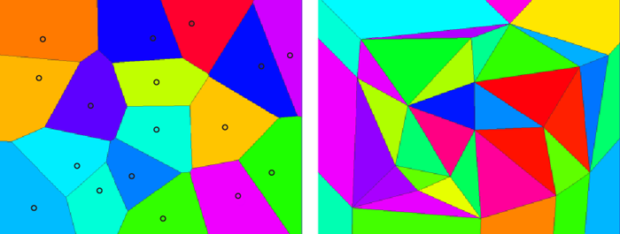
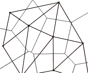
Natural neighbor interpolation is a smoothing technique that allows for surrounding sample information to contribute to the estimation of values at unsampled points. The natural neighbor method is based on Thiessen polygons (or Voronoi cells) constructed from the set of sampling locations. For any point, its natural neighbors are the locations associated with the adjacent Thiessen polygons (ESRI 2012). The values of the unsampled points are estimated using a weighted average of the values of their natural neighbors using associated polygon areas for the weights. Figure 58 illustrates the Voronoi diagrams and Figure 59 illustrates Delaunay triangles with Voronoi cells; see also the relationship between Voronoi diagrams and Delaunay triangles.

Typical Applications

▼Read more

Typical applications of this method include creating map surfaces to graphically display various properties of a data set. This method can also be used to estimate concentrations at unknown points by assuming a smooth concentration continuum between measured and unmeasured points.

Using This Method

▼Read more

This method yields the best results when a point lies within a roughly spherical set of evenly spaced natural neighbors. Smoothness of concentration changes with distance between points. A sufficient amount of data is required to understand variability in concentration. See Table 1 for more information about determining the minimum data requirements. Many software packages use this method of interpolation.

Assumptions

▼Read more

When data points are distributed in space, they inherently represent a certain area around them.

It is assumed that the sample points in sparsely sampled regions have a larger area of influence than those in the more densely sampled areas.

Strengths and Weaknesses

▼Read more


The strengths of this method are:
  • It is conceptually simple.
  • It handles large data sets well.
  • It handles highly anisotropic data sets well due to the flexibility of the polygon shapes.

The weaknesses of this method are:

    • Density of sampling points determines the size of Voronoi polygons, and thereby the inferred area of influence. Therefore, sampling density may result in misleading inferences and as with any method, this implication should be evaluated for its practical effect on accuracy.
    • Results are poor when areas of interest are around the edges of the surface, because the method does not take into account the behavior of the data, it only takes an average of the points available.
    • This method does not extrapolate contours beyond the convex hull, or boundaries, of data locations.

Understanding the Results

▼Read more

Verify results from this method by withholding known data (validation subset) from the estimation process then checking the estimated values against the known values. Field verification can be performed by collecting samples at the estimated points and determining if difference between the estimated value and data value are consistent with the CSM and reasonable to support the optimization question for the site.

Natural neighbor interpolation is often confused with nearest neighbor gridding, which is a separate method. Nearest neighbor gridding works by assigning the value of the nearest data point to each grid node (Golden Software 2002). As the value is assigned and not interpolated, nearest neighbor is more accurately described as a gridding method instead of an interpolation method. Nearest neighbor can reliably convert scattered data points to an evenly distributed sampling grid. This makes the method useful for applications such as converting one type of grid to another format (for example, an ESRI grid to a Surfer grid).

As nearest neighbor does not interpolate between data points, it should not be used for sparse data sets or to create contour lines for most environmental data sets. Where data are not on a dense grid, nearest neighbor creates polygons of uniform values and the resulting contour lines are not usable. A comparison of natural neighbor interpolation and nearest neighbor gridding results are shown on Figure 60 using the same data set as Figure 8 .

gro_fig_8_3

Figure 60. (Left) Natural neighbor interpolation results; (Right) Nearest neighbor interpolation results for the same data set, contoured at the same interval. The steep changes in values result in closely spaced contour lines in the nearest neighbor figure.

Using Analysis Results for Optimization describes how to apply the results of the geospatial methods to address specific optimization questions.

Further Information

▼Read more


The State Road 114 Superfund Site Monitoring Optimization case study uses the Voronoi/Delaunay mesh method.

Additional references include de Smith, Goodchild, and Longley 2015; Sukumar 1997; and ESRI 2012.

image_pdfPrint this page/section


GRO

web document
glossaryGRO Glossary
referencesGRO References
acronymsGRO Acronyms
ITRC
Contact Us
About ITRC
Visit ITRC
social media iconsClick here to visit ITRC on FacebookClick here to visit ITRC on TwitterClick here to visit ITRC on LinkedInITRC on Social Media
about_itrc
Permission is granted to refer to or quote from this publication with the customary acknowledgment of the source (see suggested citation and disclaimer). This web site is owned by ITRC • 1250 H Street, NW • Suite 850 • Washington, DC 20005 • (202) 266-4933 • Email: [email protected] • Terms of Service, Privacy Policy, and Usage Policy ITRC is sponsored by the Environmental Council of the States.