• Skip to main content
itrc_logo

Geospatial Analysis for Optimization at Environmental Sites

Home
About ITRC
Navigating this Website
Overview
Fact Sheets
Fact Sheets Overview
Fact Sheet 1: Do You Need Geospatial Analysis?
Fact Sheet 2: Are Conditions Suitable for Geospatial Analysis?
Fact Sheet 3: How is Geospatial Analysis Applied?
Fact Sheet 4: What Software is Available to Help?
PM's Tool Box
PM's Tool Box Overview
Review Checklist
Choosing Methods
Common Misapplications
Optimization Questions
Geospatial Analysis Support for Optimization Questions in the Project Life Cycle
Data Requirements
General Considerations
Methods for Optimization
Geospatial Methods for Optimization Questions in the Project Life Cycle Stages
Release Detection
Site Characterization
Remediation
Monitoring
Closure
Documenting Results
Fundamental Concepts
Fundamental Concepts for Geospatial Analysis
Basic Data Concepts for Geospatial Analysis
Interpolation Methods and Model Prediction
Uncertainty in Geospatial Analyses
Characteristics of Interpolation Methods
Work Flow
Work Flow for Conducting Geospatial Analysis
Geospatial Analysis Work Flow Overview
Perform Exploratory Data Analysis
Select Geospatial Method
Build Geospatial Model
Evaluate Geospatial Method Accuracy
Generate Geospatial Analysis Results
Using Results
Using Analysis Results for Optimization
Plume Intensity and Extent
Trend Maps
Estimating Quantities
Hot Spot Detection
Sample Spacing
Estimating Concentrations Based on Proxy Data
Background Estimation
Quantifying Uncertainty
Remedial Action Optimization
Monitoring Program Optimization
Examples
Examples Overview
Example 1
Example 2
Example 3
Example 4
Methods
Methods Overview
Simple Geospatial Methods
More Complex Geospatial Methods
Advanced Methods
Index of Methods
Software
Software Overview
Software Comparison Tables
Software Descriptions
Workshops and Short Courses
Case Studies
Case Studies Overview
Superfund Site Monitoring Optimization (MAROS)
PAH Contamination in Sediments—Uncertainty Analysis (Isatis)
Optimization of Long-Term Monitoring at Former Nebraska Ordnance Plant (GTS; Summit Envirosolutions)
Optimization of Lead-Contaminated Soil Remediation at a Former Lead Smelter (EVS/MVS)
Extent of Radiological Contamination in Soil at Four Sites near the Fukushima Daiichi Power Plant, Japan (ArcGIS)
Optimization of Groundwater Monitoring at a Research Facility in New Jersey (GWSDAT)
Optimization of Sediment Sampling at a Tidally Influenced Site (ArcGIS)
Stringfellow Superfund Site Monitoring Optimization (MAROS)
Lead Contamination in Soil (ArcGIS)
Stakeholder Perspectives
Additional Information
Project Life Cycle Stages
History of Remedial Process Optimization
Additional Resources
Acronyms
Glossary
Index of Methods
Acknowledgments
Team Contacts
Document Feedback


Geospatial Analysis for Optimization at Environmental Sites
HOME

Basic Data Concepts for Geospatial Analysis

Geospatial analyses assume that sample points close to one another are more related than sample points separated by a greater distance.

▼Read more

In order to generate useful maps (for example, contaminant contour maps), these methods require that the data exhibit a spatial or temporal relationship. Depending on the method employed, these relationships are either implicitly understood or explicitly quantified. Each geospatial method is also unique according to its assumptions. Simple geospatial methods make no assumptions and are therefore more relaxed in terms of their use and application. More complex and advanced methods do make statistical assumptions about the data; these assumptions are method specific and vary in their strictness. Practitioners must have a basic understanding of these assumptions in order to make informed decisions about which method is best for a given data set. The concepts covered in this section include (1) spatial dependence and autocorrelation; (2) sampling geospatial data; and (3) advanced geospatial model assumptions.

Spatial Dependence and Autocorrelation

Environmental properties and processes are typically related to one another in space, time, or both, making it possible to draw meaning out of environmental data. Environmental properties and processes follow Tobler’s First Law of Geography (Tobler 1970), which states: “Everything is related to everything else, but near things are more related than distant things.” This law means that sample observations that are collected close together in space or time are more related than sample observations collected farther apart. In a spatial context, the relationship between sample locations imparts meaning in a map, whether it is a geologic map or a three-dimensional visualization of a contaminant plume. Sampled data that relate to one another in space or time are called dependent data.

▼Read more

Autocorrelation is an explicit measure of the relationship, or correlation, between sampled data in space or time. Autocorrelation can be an expression of a single data set and illustrate how a sampled property or process relates to itself in space or time. On another level, autocorrelation can be an expression between multiple data sets (multivariate) and illustrate how multiple sampled properties or processes relate to one another in space or time; see Sampling Geospatial Data.

Advanced methods are based on the general assumption that the mean, variance, and autocorrelation properties are statistically the same over some distance ranging from some limited distance between sample points to the entire site (or sampling domain). This statistical sameness is termed “stationarity” and is discussed in more detail in Advanced Geospatial Model Assumptions.

The tools for evaluation of autocorrelation such as the variogram require selection of a value for the lag. The separation distance between two points, commonly referred to as the lag, is defined by the sampling frequencies (time and number) or grid spacing (distance and space). Thus, it is important to develop well-designed sampling programs for assessing autocorrelation. When samples are located on a sampling grid, the grid spacing is usually a good indicator for the value of the lag. If the data are acquired using an irregular or random sampling scheme, however, the selection of a suitable lag distance value is more complex. The lag value selected can affect autocorrelation. For example, if the lag value is too large, then  autocorrelation over short distances may be masked. If the lag value is too small, then groups of data points (called “bins”) will not reflect representative data averages. See Variograms for more information.

Sampling Geospatial Data

To perform geospatial analyses, the sampling program must adequately capture the dependence or autocorrelation of the properties being sampled. This design is difficult for complex systems, such as groundwater or soil environments. Consequently, site reconnaissance efforts or phased sampling programs can help to ensure that the right quantity and quality of data are being sampled. These data are assessed using the geospatial work flow steps. If preliminary analyses of these data indicate that the data are inadequate, geospatial analysis can be used to optimize sampling to determine additional sample locations.

▼Read more

Fundamental concepts for designing a sampling program to collect geospatial data include sample support, sample extent, and sample interval, which are referred to in some cases as the scale-triplet (Zhang 2011). Sample support is the area or volume represented by each observation point. Sampling extent is the observation domain or area of study. Sampling interval is the sampling distance or frequency data are collected.

A project’s sampling design should be based on the typical scales of autocorrelation exhibited by the properties being sampled. The scales of spatial autocorrelation can be local or regional, and may vary according to sampling interval and extent. For instance, to interpolate hydraulic conductivity of soil to quantify transport behavior of contaminants, the spatial sampling interval should be smaller to capture the smaller scale autocorrelation inherent in soil porosity. By comparison, to model the surface transport of pesticides across an agricultural region, the sampling interval should be relatively larger to capture regional scale autocorrelation in topographic landforms and agricultural activity affecting the transport of pesticides. Sampling interval applies to time as well. For example, when monitoring the attenuation of a recalcitrant hydrocarbon in slow moving groundwater, the temporal sampling interval can be longer than would be selected for hydrocarbons in fast moving groundwater.

Advanced Geospatial Model Assumptions

The defining feature of advanced geospatial methods is that they are based on an explicit model of spatial autocorrelation. This model must be estimated from the data. In order for this estimation to be possible, it is assumed that the statistical properties of the population from which the data are sampled do not change in space (or time). In other words, we must assume that the mean, variance, and autocorrelation do not vary in space or time (translation invariant). This assumption is called stationarity.

Advanced geospatial methods are based on the assumption that the observed data are a realization (or possible outcome) of an autocorrelated random variable. The assumption of stationarity applies to this random variable that is the basis of the advanced methods. This section describes types of stationarity as they relate to the use of advanced geospatial methods. These concepts are key for helping practitioners decide whether stationary or nonstationary advanced geospatial methods apply.

Stationarity –The assumption that the statistical properties of the population do not change over time or space. There are several types of stationarity depending on which statistical properties are assumed to be invariant over time and space. Stationarity is an important assumption for advanced geospatial methods because it allows data from different locations or times to be combined together to estimate an overall model of spatial correlation.

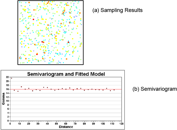
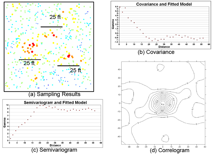
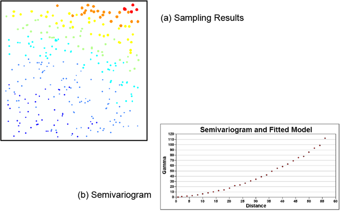
The following examples of stationarity were developed using the SAS tutorial data set. The data set has been rearranged, so the resulting data for the figures presented here are not exactly the same as the figures that would be generated directly from the SAS tutorial data set. On these figures, the concentration of a sampling point is noted by both the size of the dot and its color. The red, orange, and yellow dots have higher concentrations, with red being the highest concentrations.

Strict stationarity ▼Read more

Strict stationarity assumes that all statistical properties, including the mean, variance, skewness, and kurtosis, remain unchanged across the entire site with space or time. In the real world, this assumption means that the site or location is homogeneous across the entire sampling area. Chilès and Delfiner (1999) compare strict stationarity to a jar of well-sorted sand: the jar of sand is the sampling domain and the well-sorted sand represents homogeneity. Spatial data rarely meet the assumption of strict stationarity in their raw form, but may after transformation or detrending, or both. Figure 8 illustrates data that meet strict stationarity. A pure nugget effect, indicating a lack of spatial correlation, is illustrated in plan view in (a) and demonstrated by the nearly horizontal line of semivariance (noted as gamma on the figure) verses distance in (b), starting at a distance of zero.

gro_stationarity_fig_1_no_headline

Figure 8. Data meeting strict stationarity.

Second-order stationarity ▼Read more

Second-order stationarity requires only that the mean and covariance do not change over space or time. Second-order stationarity is also called “weak” stationarity. A random function is called second-order stationary when the mean and variance are constant and the covariance or variogram depends only on lag distance and not on absolute positions. If the distribution is normal (Gaussian), a second-order stationary random variable also meets strict stationarity. Figure 9 illustrates data that meet second-order stationarity. If a data set is second-order stationary, then intrinsic stationarity is implied (see below); however, if the data are intrinsically stationary, they are not necessarily second-order stationary.

gro_stationarity_fig_2_no_headline

Figure 9. Data meeting second-order stationarity.

Illustrated in plan view in (a), the concentrations at the sampling points, as noted by both the size of the dot and its color, are not distributed uniformly. The change in concentration versus distance can be examined by investigating the covariance (b) or semivariogram (c).  The covariance model illustrates the joint variation between all the pairs of points. The semivariogram is based on the absolute difference between the sample observations separated by the lag. If the mean is constant and the covariance independent of location, then the covariance and semivariance are mirror-images of one another as shown in the correlogram (d).

Intrinsic stationarity ▼Read more

Intrinsic stationarity assumes that for every vector (h), the linear increment of a variable is a stationary random function. In other words, the mean and variogram do not change over space (or time). The variogram measures half the variance of the differences in values measured between all possible observation points that are spaced a lag distance apart. A figure illustrating intrinsically stationarity data would look similar to one illustrating non-stationary data (Figure 10). The only way to distinguish between the two types would be to examine the local statistics of the data set.

The variogram of an intrinsically stationary dataset (that is not second-order stationary) does not exhibit a sill value.

The stationarity assumptions must be assessed to support the choice and use of advanced geospatial methods.

Nonstationary data sets ▼Read more

The simplest form of a nonstationary data set is characterized by a mean that exhibits a trend in space or time (Figure 10).

gro_stationarity_fig_3_no_headline

Figure 10. Nonstationary data.

If the data show a trend, as illustrated in plan view in (a), then the semivariogram does not stabilize at a sill but rather continues to climb (b). In this case, the concentration of the sample cannot be predicted based on lag distance.

Groundwater data sets, containing either concentrations or elevation values, often exhibit a trend or gradient, which is a good example of a nonstationary mean. On the other hand, if groundwater data are collected for multiple years, then the data typically demonstrates a seasonally repeating pattern which may have a mean that stabilizes.

The Work Flow section includes discussion of spatial exploratory data analysis and developing the empirical variogram for a data set. In addition, see the spatial correlation models for advanced geospatial methods section which discusses the theoretical variogram models used to describe spatial correlation.

image_pdfPrint this page/section


GRO

web document
glossaryGRO Glossary
referencesGRO References
acronymsGRO Acronyms
ITRC
Contact Us
About ITRC
Visit ITRC
social media iconsClick here to visit ITRC on FacebookClick here to visit ITRC on TwitterClick here to visit ITRC on LinkedInITRC on Social Media
about_itrc
Permission is granted to refer to or quote from this publication with the customary acknowledgment of the source (see suggested citation and disclaimer). This web site is owned by ITRC • 1250 H Street, NW • Suite 850 • Washington, DC 20005 • (202) 266-4933 • Email: [email protected] • Terms of Service, Privacy Policy, and Usage Policy ITRC is sponsored by the Environmental Council of the States.