• Skip to main content
itrc_logo

Geospatial Analysis for Optimization at Environmental Sites

Navigating this Website
Overview
Fact Sheets
Fact Sheets Overview
Fact Sheet 1: Do You Need Geospatial Analysis?
Fact Sheet 2: Are Conditions Suitable for Geospatial Analysis?
Fact Sheet 3: How is Geospatial Analysis Applied?
Fact Sheet 4: What Software is Available to Help?
PM's Tool Box
PM's Tool Box Overview
Review Checklist
Choosing Methods
Common Misapplications
Optimization Questions
Geospatial Analysis Support for Optimization Questions in the Project Life Cycle
Data Requirements
General Considerations
Methods for Optimization
Geospatial Methods for Optimization Questions in the Project Life Cycle Stages
Release Detection
Site Characterization
Remediation
Monitoring
Closure
Documenting Results
Fundamental Concepts
Fundamental Concepts for Geospatial Analysis
Basic Data Concepts for Geospatial Analysis
Interpolation Methods and Model Prediction
Uncertainty in Geospatial Analyses
Characteristics of Interpolation Methods
Work Flow
Work Flow for Conducting Geospatial Analysis
Geospatial Analysis Work Flow Overview
Perform Exploratory Data Analysis
Select Geospatial Method
Build Geospatial Model
Evaluate Geospatial Method Accuracy
Generate Geospatial Analysis Results
Using Results
Using Analysis Results for Optimization
Plume Intensity and Extent
Trend Maps
Estimating Quantities
Hot Spot Detection
Sample Spacing
Estimating Concentrations Based on Proxy Data
Background Estimation
Quantifying Uncertainty
Remedial Action Optimization
Monitoring Program Optimization
Examples
Examples Overview
Example 1
Example 2
Example 3
Example 4
Methods
Methods Overview
Simple Geospatial Methods
More Complex Geospatial Methods
Advanced Methods
Index of Methods
Software
Software Overview
Software Comparison Tables
Software Descriptions
Workshops and Short Courses
Case Studies
Case Studies Overview
Superfund Site Monitoring Optimization (MAROS)
PAH Contamination in Sediments—Uncertainty Analysis (Isatis)
Optimization of Long-Term Monitoring at Former Nebraska Ordnance Plant (GTS; Summit Envirosolutions)
Optimization of Lead-Contaminated Soil Remediation at a Former Lead Smelter (EVS/MVS)
Extent of Radiological Contamination in Soil at Four Sites near the Fukushima Daiichi Power Plant, Japan (ArcGIS)
Optimization of Groundwater Monitoring at a Research Facility in New Jersey (GWSDAT)
Optimization of Sediment Sampling at a Tidally Influenced Site (ArcGIS)
Stringfellow Superfund Site Monitoring Optimization (MAROS)
Lead Contamination in Soil (ArcGIS)
Stakeholder Perspectives
Additional Information
Project Life Cycle Stages
History of Remedial Process Optimization
Additional Resources
Acronyms
Glossary
Index of Methods
Acknowledgments
Team Contacts
Document Feedback


Geospatial Analysis for Optimization at Environmental Sites
HOME

Generate Geospatial Analysis Results

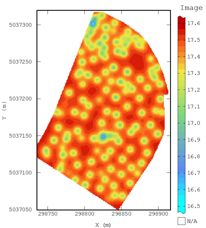
Once selected, the appropriate geospatial method is used to generate information for optimization. The type of results can vary depending on the study question being addressed, but the results usually include a set of predictions at unsampled locations and, for some methods, a measure of prediction uncertainty (such as standard errors or variances). If the geospatial method is being used to optimize a sampling plan, then the output of the method might be a proposed sampling plan or a metric that can be used to select new sampling locations or to remove existing sampling locations.

▼Read more

Many optimization tasks depend on assessing or minimizing the prediction uncertainty. Geospatial methods differ in their ability to provide quantitative measures of uncertainty for predictions at unsampled locations. The simple methods do not provide any form of statistical uncertainty estimates. For these methods, uncertainty in the predicted values can only be evaluated qualitatively by considering whether the results are consistent with the CSM and whether the available data are sufficient to answer the questions of interest.

More complex methods, such as regression and spatial correlation approaches, use standard probability theory to quantify uncertainty. Since spatial regression models include a statistical noise or error term, this method can be used to quantify uncertainty in the model predictions as with a regular, nonspatial regression model. However, the estimates of uncertainty from spatial regression models may be underestimated if spatial correlation is not fully accounted for. In principle, methods such as kriging, which account for spatial correlation, may produce better estimates of prediction uncertainty. The uncertainty estimates from kriging are also too low because they generally do not include the uncertainty associated with estimating the parameters of the spatial correlation model.

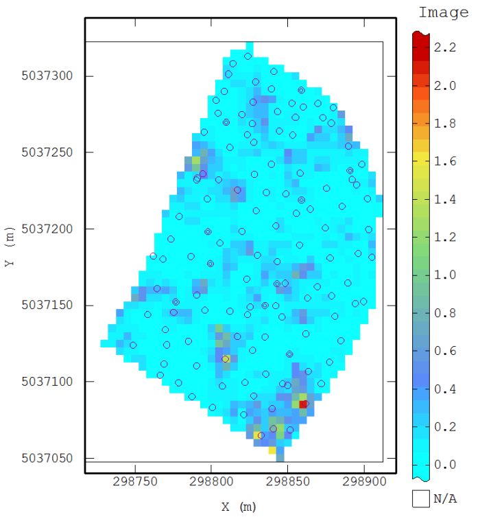
The uncertainty in the geospatial method results can be visualized by plotting the prediction variance (from regression or kriging methods) or statistical summaries of the results of conditional simulation. The most common ways of characterizing uncertainty are described in more detail in the following subsections.

Variance Map

▼Read more

The prediction standard error or variance provides an estimate of the interpolation accuracy that can be generated by more complex and advanced methods. This measure of uncertainty can be mapped in order to show areas of greater and lesser uncertainty. The map can be used qualitatively or quantitatively for the optimization of sampling plans. For some kriging methods, the standard errors depend only on the sample locations, estimated variogram, and kriging method, but not on the measured values at sampling locations. These conditions simplify the use of these methods for sampling plan optimization. Figure 48 shows an example of a prediction variance map generated from kriging.

gro_wf_23

Figure 48. Example of a prediction variance map generated using kriging.

The most accurately estimated areas correspond to sampling points where the value is exactly known (blue areas). The interpolation is less reliable in areas, where no samples have been collected (red areas).

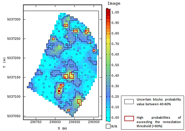
Statistical and Probability Maps

▼Read more

Conditional simulation provides a method to more completely quantify the uncertainties of the estimates. Interpolation using conditional simulation can produce maps of the contamination which are based on the input data, the estimated variogram, and the kriging model. The maps are all equally probable and conditioned on the observed values at each location. The maps are consistent with both first order statistics (histogram) and the second order statistics (variogram). Postprocessing of conditional simulations (compilation of all equally probable maps) can produce two types of maps that can help to analyze the degree of uncertainty of the estimate: a standard deviation map (Figure 49A) and a probability map (Figure 49B).

Standard Deviation Map

▼Read more

A standard deviation map quantifies the standard deviation at each block, taking into account the values measured at each sampling location. Figure 49A shows an example standard deviation map.

gro_wf_24

Figure 49A. Example of a prediction standard deviation map generated using conditional simulation.

Probability Map

▼Read more

It is possible to estimate the certainty that the average concentration in a block exceeds the cleanup level. These maps are expressed in terms of the probability of exceeding the cleanup level. Figure 49B is an example probability map.

gro_wf_25

Figure 49B. Example of a prediction exceedance probability map generated using conditional simulation.

The blue blocks correspond to probabilities of exceeding the threshold that are lower than 25%. These are the areas where the risk of contamination is low. On the other hand, yellow and red zones correspond to high probabilities of exceeding the remediation threshold (above 60%) and may represent potential contaminant source areas. Particular attention should be paid to the green blocks corresponding to the uncertain areas. These blocks have a probability of exceeding the remediation threshold between 40% and 60% (fifty-fifty chance of exceeding the threshold). These blocks represent areas where the information about the occurrence of contamination is less accurate. Quantifying these uncertain blocks allows a better understanding of the uncertain volume in order to manage the risks of the remediation.

image_pdfPrint this page/section


GRO

web document
glossaryGRO Glossary
referencesGRO References
acronymsGRO Acronyms
ITRC
Contact Us
About ITRC
Visit ITRC
social media iconsClick here to visit ITRC on FacebookClick here to visit ITRC on TwitterClick here to visit ITRC on LinkedInITRC on Social Media
about_itrc
Permission is granted to refer to or quote from this publication with the customary acknowledgment of the source (see suggested citation and disclaimer). This web site is owned by ITRC • 1250 H Street, NW • Suite 850 • Washington, DC 20005 • (202) 266-4933 • Email: [email protected] • Terms of Service, Privacy Policy, and Usage Policy ITRC is sponsored by the Environmental Council of the States.