• Skip to main content
itrc_logo

Geospatial Analysis for Optimization at Environmental Sites

Navigating this Website
Overview
Fact Sheets
Fact Sheets Overview
Fact Sheet 1: Do You Need Geospatial Analysis?
Fact Sheet 2: Are Conditions Suitable for Geospatial Analysis?
Fact Sheet 3: How is Geospatial Analysis Applied?
Fact Sheet 4: What Software is Available to Help?
PM's Tool Box
PM's Tool Box Overview
Review Checklist
Choosing Methods
Common Misapplications
Optimization Questions
Geospatial Analysis Support for Optimization Questions in the Project Life Cycle
Data Requirements
General Considerations
Methods for Optimization
Geospatial Methods for Optimization Questions in the Project Life Cycle Stages
Release Detection
Site Characterization
Remediation
Monitoring
Closure
Documenting Results
Fundamental Concepts
Fundamental Concepts for Geospatial Analysis
Basic Data Concepts for Geospatial Analysis
Interpolation Methods and Model Prediction
Uncertainty in Geospatial Analyses
Characteristics of Interpolation Methods
Work Flow
Work Flow for Conducting Geospatial Analysis
Geospatial Analysis Work Flow Overview
Perform Exploratory Data Analysis
Select Geospatial Method
Build Geospatial Model
Evaluate Geospatial Method Accuracy
Generate Geospatial Analysis Results
Using Results
Using Analysis Results for Optimization
Plume Intensity and Extent
Trend Maps
Estimating Quantities
Hot Spot Detection
Sample Spacing
Estimating Concentrations Based on Proxy Data
Background Estimation
Quantifying Uncertainty
Remedial Action Optimization
Monitoring Program Optimization
Examples
Examples Overview
Example 1
Example 2
Example 3
Example 4
Methods
Methods Overview
Simple Geospatial Methods
More Complex Geospatial Methods
Advanced Methods
Index of Methods
Software
Software Overview
Software Comparison Tables
Software Descriptions
Workshops and Short Courses
Case Studies
Case Studies Overview
Superfund Site Monitoring Optimization (MAROS)
PAH Contamination in Sediments—Uncertainty Analysis (Isatis)
Optimization of Long-Term Monitoring at Former Nebraska Ordnance Plant (GTS; Summit Envirosolutions)
Optimization of Lead-Contaminated Soil Remediation at a Former Lead Smelter (EVS/MVS)
Extent of Radiological Contamination in Soil at Four Sites near the Fukushima Daiichi Power Plant, Japan (ArcGIS)
Optimization of Groundwater Monitoring at a Research Facility in New Jersey (GWSDAT)
Optimization of Sediment Sampling at a Tidally Influenced Site (ArcGIS)
Stringfellow Superfund Site Monitoring Optimization (MAROS)
Lead Contamination in Soil (ArcGIS)
Stakeholder Perspectives
Additional Information
Project Life Cycle Stages
History of Remedial Process Optimization
Additional Resources
Acronyms
Glossary
Index of Methods
Acknowledgments
Team Contacts
Document Feedback


Geospatial Analysis for Optimization at Environmental Sites
HOME

Closure

The primary aim of closure stage is to use sampling data to ensure that the site no longer needs monitoring, or that it may be transitioned to other land uses. In many cases, using geospatial analysis can be limited by the lack of contaminant detections at the site at closure, particularly where the cleanup goals are close to the analytical detection limits.

Closure is the final stage of the life cycle in which the determination is made about whether to permanently cease monitoring. Geospatial methods can support closure through:

  • demonstrating compliance with criteria
  • demonstrating acceptable trends toward achieving compliance criteria
  • supporting methods for determining closure objectives by
    • modeling using collected data
    • conducting uncertainty analyses to account for uncertainty in goals and objectives
    • preparing visual representations of site conditions
  • retaining geospatial data and management procedures for the final administrative record (including the model used, model assumptions, data used and output files)
  • reducing costs by demonstrating successful mass removal and acceptable trends (as discussed in Monitoring)

Figure 7 provides an overview of the role of geospatial methods in this stage of the project life cycle. Each general topic, specific question, and method is linked to a more detailed discussion.

Figure 7

Click Here to go to Attainment of Closure Goals Click Here to go to Plume Change/Attenuation Over Time Click Here to go to Trend Maps Click Here to go to Monitoring Program Optimization

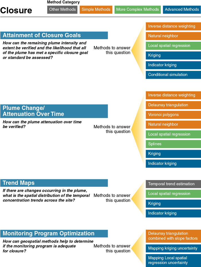
Figure 7. Closure overview.

Closure: Attainment of Closure Goals

How can the remaining plume intensity and extent be verified and the likelihood that all of the plume has met a specific closure goal or standard be assessed?

▼Read more

Because they include spatial mapping of measurement data, geospatial methods serve as an alternative to professional judgment or hand contouring when creating site maps. Such maps are necessary to ensure the plume is attenuating over time or is projected not to exceed regulatory limits in the future. One of the closure goals may be to achieve a stable or shrinking plume. In this case, the spatial analysis of trends may be appropriate and the analysis is discussed with other questions below. For more information, see the discussion on using geospatial results in quantifying uncertainty.

Geospatial Methods:

  1. Simple geospatial methods can be used for mapping, including inverse distance weighting, natural neighbor interpolation and similar methods can be used to map the plume.
  2. More complex geospatial methods, including local spatial regression, can also estimate the potential uncertainty in the values.
  3. Kriging, including indicator kriging, can be used to estimate likelihood that areas have attained the closure standard.
  4. Other advanced methods such as conditional simulation can be performed. Conditional simulation uses the spatial correlation relationships in order to assess the probabilities that the plume is below a cleanup goal.

Closure: Plume Change/Attenuation Over Time

How can the plume attenuation over time be verified?

▼Read more

As with monitoring, plume evaluation is also part of the closure stage, only with a focus on the successful approach toward goals. The change in concentrations can be assessed at individual sampling locations, but the plume as a whole cannot be tracked without spatial mapping of the plume at a series of points through time. A series of geospatial plume maps at distinct times can be compared to assess changes in extent or intensity. If many of the values are nondetect, the available methods may be limited. For more information, see the discussion on using geospatial results in estimating quantities.

Geospatial Methods:

  1. Simple geospatial methods, including inverse distance weighting, Delaunay triangulation with Voronoi polygons, and natural neighbor interpolation, can also be used on mutually exclusive subsets of the data representing distinct time periods or sampling events to assess plume changes.
  2. More complex geospatial methods, such as local spatial regression and splines can also be used.
  3. Advanced methods such as kriging can be used, including indicator kriging where the indicator would be for the change over time (for example, increasing or decreasing values). Note that indicator kriging can address nondetect concentrations, provided the detection limits are below the concentration goal.

Closure: Trend Maps

If there are changes occurring in the plume, what is the spatial distribution of the temporal concentration trends across the site?

▼Read more

As in the monitoring stage, closure trend maps represent a summary method of tracking plume change and attenuation over time. Instead of mapping the plume at a series of time points, the slope direction and magnitude is estimated at each sampling location and then plotted on a site map. A trend map thus provides a spatial overview of which areas of the site are increasing or decreasing in concentration, as well as how quickly. For closure, the trends should be decreasing or stable with concentrations below the applicable closure threshold. The rate of decline may be useful to assess the time to attainment of closure goals. Again, a large fraction of nondetected concentrations may pose a limitation to many of these methods. For more information on using geospatial results in understanding trends, see Trend Maps.

Geospatial Methods:

  1. Temporal trend estimation (linear regression, Mann-Kendall, Theil-Sen) can be combined with plotting of the magnitude and direction of the trends on a map. The GSMC-1 document (ITRC 2013) includes more information on trend estimation methods.
  2. More complex methods (for example, local spatial regression) can be used to interpolate the data over both space and time to provide a series of plume maps at different times.
  3. Kriging, including indicator kriging, can be used to map the likely distribution of the determined trend. The statistical confidence in the trend (positive values for increasing trends and negative values for a decreasing trend) can be kriged, or indicator kriging can be used to evaluate certainty of trends by assigning a one to an increasing trend and a zero to the opposite trend.

Closure: Monitoring Program Optimization

How can geospatial methods help to determine if the monitoring program is adequate for closure?

▼Read more

Assessing monitoring program adequacy is similar to the monitoring program optimization conducted in the monitoring stage. These methods can help to determine whether the current number and arrangement of sampling locations is adequate to accurately track plume extent and intensity relative to closure goals. A map of the spatial uncertainty can be estimated to locate particular site areas where new sampling locations might be needed or desirable to reduce local uncertainty. For more information, see the discussion of using geospatial results in monitoring program optimization.

Geospatial Methods:

  1. Delaunay triangulation with interpolation of slope factors to unsampled site areas can be used to estimate uncertainty. Slope factors, as used in the MAROS software, can be used to rank wells in terms of importance for mapping the plume.
  2. Mapping of kriging uncertainty or local spatial regression uncertainty can determine local site areas where new sampling locations might be needed to enable better evaluation of closure status.

image_pdfPrint this page/section


GRO

web document
glossaryGRO Glossary
referencesGRO References
acronymsGRO Acronyms
ITRC
Contact Us
About ITRC
Visit ITRC
social media iconsClick here to visit ITRC on FacebookClick here to visit ITRC on TwitterClick here to visit ITRC on LinkedInITRC on Social Media
about_itrc
Permission is granted to refer to or quote from this publication with the customary acknowledgment of the source (see suggested citation and disclaimer). This web site is owned by ITRC • 1250 H Street, NW • Suite 850 • Washington, DC 20005 • (202) 266-4933 • Email: [email protected] • Terms of Service, Privacy Policy, and Usage Policy ITRC is sponsored by the Environmental Council of the States.