• Skip to main content
itrc_logo

Geospatial Analysis for Optimization at Environmental Sites

Home
About ITRC
Navigating this Website
Overview
Fact Sheets
Fact Sheets Overview
Fact Sheet 1: Do You Need Geospatial Analysis?
Fact Sheet 2: Are Conditions Suitable for Geospatial Analysis?
Fact Sheet 3: How is Geospatial Analysis Applied?
Fact Sheet 4: What Software is Available to Help?
PM's Tool Box
PM's Tool Box Overview
Review Checklist
Choosing Methods
Common Misapplications
Optimization Questions
Geospatial Analysis Support for Optimization Questions in the Project Life Cycle
Data Requirements
General Considerations
Methods for Optimization
Geospatial Methods for Optimization Questions in the Project Life Cycle Stages
Release Detection
Site Characterization
Remediation
Monitoring
Closure
Documenting Results
Fundamental Concepts
Fundamental Concepts for Geospatial Analysis
Basic Data Concepts for Geospatial Analysis
Interpolation Methods and Model Prediction
Uncertainty in Geospatial Analyses
Characteristics of Interpolation Methods
Work Flow
Work Flow for Conducting Geospatial Analysis
Geospatial Analysis Work Flow Overview
Perform Exploratory Data Analysis
Select Geospatial Method
Build Geospatial Model
Evaluate Geospatial Method Accuracy
Generate Geospatial Analysis Results
Using Results
Using Analysis Results for Optimization
Plume Intensity and Extent
Trend Maps
Estimating Quantities
Hot Spot Detection
Sample Spacing
Estimating Concentrations Based on Proxy Data
Background Estimation
Quantifying Uncertainty
Remedial Action Optimization
Monitoring Program Optimization
Examples
Examples Overview
Example 1
Example 2
Example 3
Example 4
Methods
Methods Overview
Simple Geospatial Methods
More Complex Geospatial Methods
Advanced Methods
Index of Methods
Software
Software Overview
Software Comparison Tables
Software Descriptions
Workshops and Short Courses
Case Studies
Case Studies Overview
Superfund Site Monitoring Optimization (MAROS)
PAH Contamination in Sediments—Uncertainty Analysis (Isatis)
Optimization of Long-Term Monitoring at Former Nebraska Ordnance Plant (GTS; Summit Envirosolutions)
Optimization of Lead-Contaminated Soil Remediation at a Former Lead Smelter (EVS/MVS)
Extent of Radiological Contamination in Soil at Four Sites near the Fukushima Daiichi Power Plant, Japan (ArcGIS)
Optimization of Groundwater Monitoring at a Research Facility in New Jersey (GWSDAT)
Optimization of Sediment Sampling at a Tidally Influenced Site (ArcGIS)
Stringfellow Superfund Site Monitoring Optimization (MAROS)
Lead Contamination in Soil (ArcGIS)
Stakeholder Perspectives
Additional Information
Project Life Cycle Stages
History of Remedial Process Optimization
Additional Resources
Acronyms
Glossary
Index of Methods
Acknowledgments
Team Contacts
Document Feedback


Geospatial Analysis for Optimization at Environmental Sites
HOME

Monitoring

The primary goal of monitoring is regular, systematic collection of sampling data in order to track measurement levels over time and to ensure that regulatory targets or limits are met. An effective monitoring program begins with a question: What is the goal of monitoring at this site? Typically, monitoring objectives fall into one or more of the following categories, all of which may be supported using geospatial methods:

  • monitoring for concentration changes
  • assessing the practicability of achieving remediation in a defined time frame
  • considering monitoring programs for each environmental medium (for example groundwater, soil, sediment)
  • assessing compliance with a criterion, standard, or regulatory requirement
  • determining whether contamination is migrating, specifically
    • determining whether contamination will reach a receptor (such as a drinking water supply well)
    • tracking the changes in shape, size, or position of a contaminant plume
  • assessing the performance of a remedial system, including monitored natural attenuation (MNA)
  • determining whether the data quality objectives (DQOs) are being met
  • validating the CSM or conclusions of a remedial investigation/feasibility study (RI/FS)
  • confirming the data evaluation, management, and reporting procedures are effective or selecting different methods, considering:
    • accuracy and precision needs
    • model demands
    • costs

Figure 6 provides an overview of the role of geospatial methods in this stage of the project life cycle. Each general topic, specific question, and method is linked to a more detailed discussion.

Figure 6 Monitoring Overview


Click Here to go to Plume Intensity and Extent Click Here to go to Plume Change/ Attenuation Over Time Click Here to go to Trend Maps Click Here to go to Monitoring Program Optimization

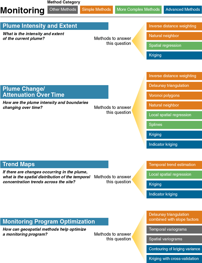
Figure 6. Monitoring overview.

Monitoring: Plume Intensity and Extent

What is the intensity and extent of the current plume?

▼Read more

Because they include spatial mapping of measurement data, geospatial methods serve as an alternative to professional judgment or hand contouring when creating the site map. The methods below provide maps that can be used to assess the plume boundaries and internal concentrations. For more information, see the discussion on using geospatial results in estimating plume intensity and extent.

Geospatial Methods:

  1. Simple geospatial methods such as inverse distance weighting, natural neighbor interpolation and other interpolation methods can be used.
  2. More complex geospatial methods such as spatial regression techniques can be used.
  3. Advanced methods – kriging of various types can also be used, depending on the nature of the data and any underlying trends.

Monitoring: Plume Change/Attenuation Over Time

How are the plume intensity and boundaries changing over time?

▼Read more

Change in concentrations can be assessed at individual sampling locations, but the plume as a whole cannot be tracked without spatial mapping of the plume at a series of points through time; a series of geospatial plume maps at distinct times can be compared to assess changes in extent or intensity. The well network must be reasonably comparable from round to round to avoid changes in the network from giving a false indication of concentration variations. This can be fundamental information for assessing optimization of the monitoring program. For more information, see the discussion of using geospatial results in estimating quantities for plume change over time.

Geospatial Methods:

  1. Simple geospatial methods such as inverse distance weighting, Delaunay triangulation with Voronoi polygons, and natural neighbor interpolation can be used on mutually exclusive subsets of the data representing distinct time periods or sampling events to assess plume changes.
  2. More complex geospatial methods such as local spatial regression and splines can be used.
  3. Advanced methods such as kriging, including indicator kriging where the indicator would be for the change over time (for example, increasing or decreasing values), can be used. Note that indicator kriging can address nondetected concentrations, provided the detection limits are below the concentration goal.

Monitoring: Trend Maps

If there are changes occurring in the plume, what is the spatial distribution of the temporal concentration trends across the site?

▼Read more

To better assess plume change over time, instead of mapping the plume at a series of time points, the slope direction and magnitude for a given parameter is estimated at each sampling location and then this information is plotted on a site map (postplotting). A trend map provides a spatial overview of which areas of the site are increasing or decreasing in concentration, as well as how quickly. This map can be useful to assess optimization of the monitoring locations and frequency. For more information, see Trend Maps.

Geospatial Methods:

  1. Temporal trend estimation (linear regression, Mann-Kendall, Theil-Sen) can be combined with plotting of the magnitude and direction of the trends on a map. The GSMC-1 document (ITRC 2013) includes more information on trend estimation methods.
  2. More complex methods (for example, local spatial regression) can be used to interpolate the data over both space and time to provide a series of plume maps at different times.
  3. Kriging, including indicator kriging, can be used to map the likely distribution of the trend. The statistical confidence in the trend (positive values for increasing trends and negative values for a decreasing trend) can be kriged, or indicator kriging can be used to evaluate certainty of trends by assigning a one to an increasing trend and a zero to the opposite trend.

Monitoring: Monitoring Program Optimization

How can geospatial methods help optimize a monitoring program?

▼Read more

During long-term groundwater monitoring, it is often helpful to periodically analyze the frequency and locations of monitoring to determine optimal sampling intervals and avoid sampling location redundancy. One strategy for determining optimal sampling intervals is to estimate a temporal variogram. Using a variogram, location redundancy can be assessed by repeated mapping of the site using a range of possible monitoring network subsets. Location redundancy can also be assessed by measuring the change in concentration uncertainty when sampling locations are temporarily removed, one-by-one, from the monitoring program. Genetic algorithms or other optimization algorithms can be used to assess the possible optimal combination of sampling locations that can be used to construct a reasonable picture of the plume, subject to constraints. Kriging or other interpolation methods are often used in conjunction with the genetic algorithms to compute a measure of the goodness of the representation based on a specific combination of sampling locations. For more information, see the discussion of using geospatial results in monitoring program optimization.

Geospatial Methods:

  1. Delaunay triangulation combined with slope factors (slope factors, as used in the MAROS software, can be used to rank wells in terms of importance for mapping the plume).
  2. Temporal variograms can be used for determining optimal sampling intervals. The temporal range at which the samples are no longer temporally correlated, is a basis for selecting a sampling frequency to reduce duplicative information. The variograms can be developed for individual wells with adequate number of sampling events (typically of higher frequency) or can be done for a larger group of wells at the site.
  3. Spatial variograms can be used to assess spatial redundancy by comparing the range of data to typical sampling location spacing.
  4. Contouring of kriging variance can be done to assess areas of high uncertainty in interpolated values as possible locations of additional monitoring.
  5. Kriging (of various kinds) with cross-validation to assess ability of other nearby points to adequately estimate values at a sampling location.

image_pdfPrint this page/section


GRO

web document
glossaryGRO Glossary
referencesGRO References
acronymsGRO Acronyms
ITRC
Contact Us
About ITRC
Visit ITRC
social media iconsClick here to visit ITRC on FacebookClick here to visit ITRC on TwitterClick here to visit ITRC on LinkedInITRC on Social Media
about_itrc
Permission is granted to refer to or quote from this publication with the customary acknowledgment of the source (see suggested citation and disclaimer). This web site is owned by ITRC • 1250 H Street, NW • Suite 850 • Washington, DC 20005 • (202) 266-4933 • Email: [email protected] • Terms of Service, Privacy Policy, and Usage Policy ITRC is sponsored by the Environmental Council of the States.