Lead Contamination in Soil (ArcGIS)
Contact: Shanna Alexander, Georgia, EPD, [email protected]
Problem Statement
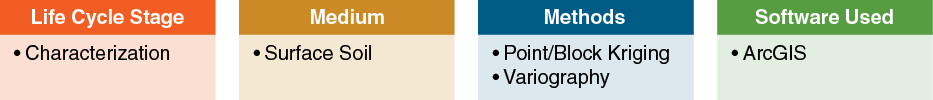
9.17-acre industrial property was characterized by urban fill present throughout the site. Urban fill presents a unique situation because there is no reasonably defined source area, but rather a widespread matrix of heterogeneous material with varying concentrations of regulated substances. The site was evaluated based upon a statistical average of predefined exposure domains in order to realistically characterize risk. Lead was the primary risk driver because of its widespread distribution in surface soil (defined as the top two feet of soil by the regulatory program).
Site Background
The site consists of 9.17 acres located Fulton County, Georgia. There are currently no operations at the site. All structures, except for an unoccupied office building, have been demolished and removed from the property, with the exception of some former building slabs. Access to the site is available via gated entries along two adjacent roadways, as well as other unfenced portions of the property. The site is relatively flat, with topographic relief to the east-southeast; however, the topography of the surrounding area has been mostly modified by urban development. Surface drainage and groundwater flow on the property mirrors the topographic relief with gradients to the southeast.
Various environmental investigations and soil removal activities were conducted, which detected lead, semivolatile organic compounds, and volatile organic compounds in the soils and groundwater on site. The site was subsequently listed on the state’s Hazardous Site Inventory because of lead values in soil above the established notification concentration of 400 mg/kg.
Project Objectives
The primary objective of the kriging analysis was to bring site concentrations of lead in soil into compliance with the established nonresidential cleanup standard of 400 mg/kg by applying a statistical “average” approach to predefined exposure domains.
Data Set
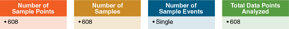
A general rule of thumb in kriging analyses is that a minimum of 30 data points is required for analysis. In this case, a total of 608 data points (fixed laboratory analysis and XRF screening) were used for kriging. The 608 data points represent the surface lead concentrations detected during several investigations. The sample population was vetted and data points which were subsequently removed during the excavations were replaced by the average lead concentrations from the fill material analyses. For the final compliance determination, surface soil data from the 0-1 ft depth range was used to determine the EPCs for each ED. As part of a sensitivity analysis, a geostatistical analysis was also completed for the soil data from the 0-2 ft depth range.
Methods
Kriging Analysis
In kriging analysis, the estimation process is governed by the spatial correlation between the data points being analyzed. The concentration of the data is determined by computing a sample variogram, which forms the basis for modeling the data and for predicting and mapping the data across the site using the process of point or block kriging. In determining the sample variogram, all pairs of measurement values in a data set are compared to each other in order to provide a consistent measure of their degree of spatial correlation. The accuracy of the kriging process is measured by the kriging standard deviation and the corresponding correlation distance (referred as the range). An example of the variogram is provided in Figure 122.
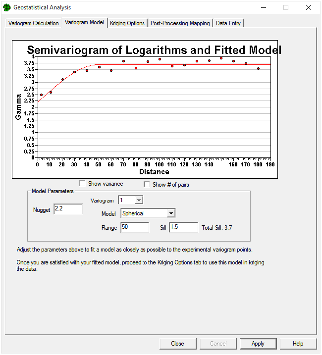 Figure 122. Example variogram in ArcGIS Geostatistical Analyst.
Selection of the Block Size (Exposure Unit)
The block sizes used for kriging depend on the specific application. Based on experience in applying kriging analysis for developing excavation plans for contaminated soils, a 30 x 30 ft block has provided optimal results for capturing the spatial extent of contamination. The size of the kriging block determines which data points influence the block estimate and the accuracy of the results.
Geospatial Analysis (Block Kriging)
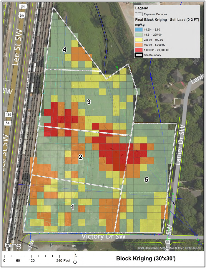 Figure 123. Current soil lead (0-2 ft, 608 samples) values were converted to block kriging (30 x 30 ft).
Source: Base map copyright 2014 Microsoft Corporation, copyright 2014 Nokia, Copyright AND
Removal of Past Excavated Areas
Replacement of excavated blocks with a value of 36 mg/Kg, which corresponds to the backfill lead concentration, is shown in Figure 124.
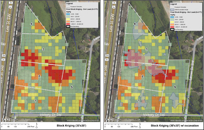 Figure 124. Block Kriging (30 x 30 ft) and Block Kriging (30 x 30 ft) with excavation.
Source: Base map copyright 2014 Microsoft Corporation, copyright 2014 Nokia, Copyright AND
Calculated 95% UCL
The 95% UCL of the mean for each domain was calculated using kriging block values for preexcavation and postexcavation.
Results
Identify Excedance Domains
The preremedy UCL and postremedy UCL for lead were calculated as shown in Figure 125 and listed in Table 16.
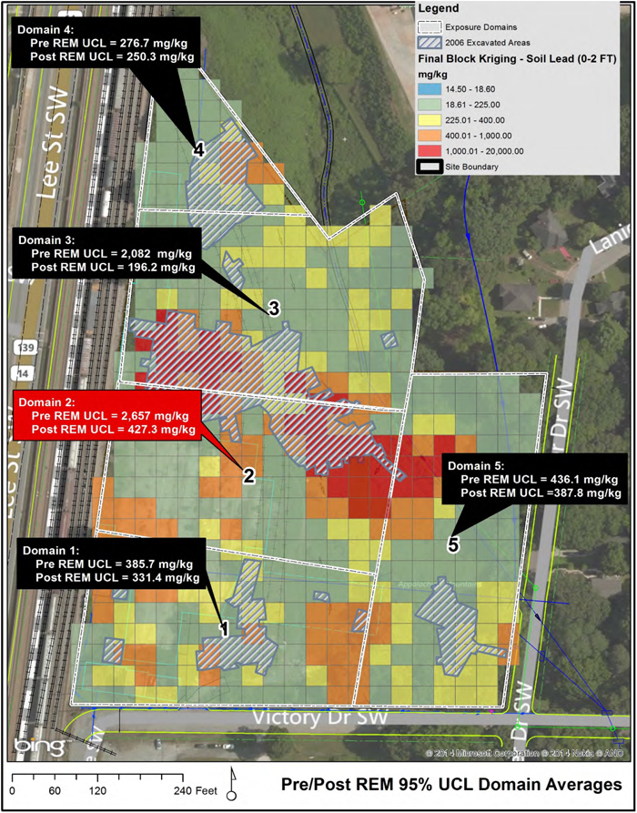 Figure 125. Pre- and Postremedy 95% UCL domain average.
Source: Base map copyright 2014 Microsoft Corporation, copyright 2014 Nokia, Copyright AND
Table 16. Pre- and Postremedy 95% UCL domain average
| Exposure Domain | Preremedy Lead (ppm) |
Postremedy Lead (ppm) |
|---|---|---|
| 1 | 331.4 | 385.7 |
| 2 | 427.3 | 2,657 |
| 3 | 196.2 | 2,082 |
| 4 | 250.3 | 276.7 |
| 5 | 387.8 | 436.1 |
Identifying Blocks Causing Domain Exceedances
Figure 125 shows the concentrations of lead in each block. This figure highlights an area with several blocks with high lead concentrations. If these blocks are removed, the UCL average can pass the remedial goal of 400 ppm. Table 17 lists lead concentrations in each Domain before and after excavations.
Table 17. Pre- and Postremedies 1 and 2 95% UCL domain average
| Exposure Domain | Preremedy Lead (ppm) |
Postremedy 1Lead (ppm) |
Postremedy 2 Lead (ppm) |
|---|---|---|---|
| 1 | 385.7 | 331.4 | NA/Same |
| 2 | 2,657 | 427.3 | 299.6 |
| 3 | 2,082 | 196.2 | NA/Same |
| 4 | 276.7 | 250.3 | NA/Same |
| 5 | 436.1 | 387.8 | NA/Same |
Actual Removal Conducted and Final UCL in Each Domain
The affected surficial (0 to 1ft) lead-contaminated soil in the on-site area identified by the kriging analysis was excavated. In addition, a voluntary off-site soil excavation was performed. A total of 73.5 tons of soil were excavated, including 5.53 tons from the off-site property. The extent of excavation of impacted soil was confirmed through postexcavation verification sampling using XRF screening with fixed laboratory confirmation analyses. The final kriging results for lead are listed in Table 18 where all 5 UCL mean values are reported below the 400 mg/kg cleanup criteria.
Table 18. Summary of final kriging results for lead by exposure domain
| Exposure Domain 95% UCL of Mean (0-1 FT) | |
|---|---|
| Domain 1 | 263.5 mg/kg |
| Domain 2 | 370.1 mg/kg |
| Domain 3 | 309.0 mg/kg |
| Domain 4 | 387.1 mg/kg |
| Domain 5 | 295.4 mg/kg |
Remediation Summary
The kriging analysis identified approximately 1,180 cubic yards of lead-impacted soils that required removal to bring the EPC in each domain into compliance with the nonresidential cleanup standard of 400 mg/kg for lead.
The total volume of soil removed was 73.4 tons, including 5.53 tons from an off-site residential property. After final excavation was completed, confirmation soil samples were collected. The results of the postexcavation confirmation sampling were used to update the kriging model. The final kriging results for lead for the five exposure domains show that all five EPC values for lead were below the cleanup standard of 400 mg/kg. A Uniform Environmental Covenant was proposed for the site in order to maintain the exposure conditions (limit direct exposure) and cleanup criteria certified within the Compliance Status Report for the site.

