• Skip to main content
itrc_logo

Geospatial Analysis for Optimization at Environmental Sites

Navigating this Website
Overview
Fact Sheets
Fact Sheets Overview
Fact Sheet 1: Do You Need Geospatial Analysis?
Fact Sheet 2: Are Conditions Suitable for Geospatial Analysis?
Fact Sheet 3: How is Geospatial Analysis Applied?
Fact Sheet 4: What Software is Available to Help?
PM's Tool Box
PM's Tool Box Overview
Review Checklist
Choosing Methods
Common Misapplications
Optimization Questions
Geospatial Analysis Support for Optimization Questions in the Project Life Cycle
Data Requirements
General Considerations
Methods for Optimization
Geospatial Methods for Optimization Questions in the Project Life Cycle Stages
Release Detection
Site Characterization
Remediation
Monitoring
Closure
Documenting Results
Fundamental Concepts
Fundamental Concepts for Geospatial Analysis
Basic Data Concepts for Geospatial Analysis
Interpolation Methods and Model Prediction
Uncertainty in Geospatial Analyses
Characteristics of Interpolation Methods
Work Flow
Work Flow for Conducting Geospatial Analysis
Geospatial Analysis Work Flow Overview
Perform Exploratory Data Analysis
Select Geospatial Method
Build Geospatial Model
Evaluate Geospatial Method Accuracy
Generate Geospatial Analysis Results
Using Results
Using Analysis Results for Optimization
Plume Intensity and Extent
Trend Maps
Estimating Quantities
Hot Spot Detection
Sample Spacing
Estimating Concentrations Based on Proxy Data
Background Estimation
Quantifying Uncertainty
Remedial Action Optimization
Monitoring Program Optimization
Examples
Examples Overview
Example 1
Example 2
Example 3
Example 4
Methods
Methods Overview
Simple Geospatial Methods
More Complex Geospatial Methods
Advanced Methods
Index of Methods
Software
Software Overview
Software Comparison Tables
Software Descriptions
Workshops and Short Courses
Case Studies
Case Studies Overview
Superfund Site Monitoring Optimization (MAROS)
PAH Contamination in Sediments—Uncertainty Analysis (Isatis)
Optimization of Long-Term Monitoring at Former Nebraska Ordnance Plant (GTS; Summit Envirosolutions)
Optimization of Lead-Contaminated Soil Remediation at a Former Lead Smelter (EVS/MVS)
Extent of Radiological Contamination in Soil at Four Sites near the Fukushima Daiichi Power Plant, Japan (ArcGIS)
Optimization of Groundwater Monitoring at a Research Facility in New Jersey (GWSDAT)
Optimization of Sediment Sampling at a Tidally Influenced Site (ArcGIS)
Stringfellow Superfund Site Monitoring Optimization (MAROS)
Lead Contamination in Soil (ArcGIS)
Stakeholder Perspectives
Additional Information
Project Life Cycle Stages
History of Remedial Process Optimization
Additional Resources
Acronyms
Glossary
Index of Methods
Acknowledgments
Team Contacts
Document Feedback


Geospatial Analysis for Optimization at Environmental Sites
HOME

Site Characterization

Site characterization describes the nature and the extent of the contamination and defines contaminant pathways and receptors. Geospatial methods can improve the efficiency of the site characterization by:

  • providing a basis for estimating the total mass and extent of contamination, including an estimate of the uncertainty in the estimate
  • improving estimation of critical contaminant statistical parameters, including exposure point concentrations
  • providing an optimized basis for sample spacing that minimizes duplicative information
  • providing for interpolation of results by considering the actual spatial correlation of the results, which allows a more complete picture of the contaminant footprint and impact and provides information on the uncertainty in the interpolated values
  • refining background data (GSMC-1) by including naturally occurring spatial variability
  • refining the CSM using data collected during the site characterization stage by:
    • employing spatial modeling or temporal modeling
    • quantifying uncertainty in contamination areal and magnitude definition (data gaps) and reducing uncertainty in CSM parameters
    • adjusting the number of monitoring points (minimum and sufficient)
    • improving spatial coverage and monitoring point placement
    • optimizing the frequency of monitoring (minimum and sufficient)
    • identifying essential data (chemical concentrations, physical parameters)
  • generating site-specific information based on physical site conditions, geology, hydrology and chemistry data
  • identifying the location of sources, number of potential sources, and relative contributions from comingled sources
  • illustrating transport pathways, groundwater dynamics (water levels, flow, and direction of flow) and plume dynamics (contaminant concentration fluctuations, shape, size, expansion or contraction, and attenuation)
  • supporting data evaluation, management, and reporting procedures by confirming sampling and monitoring methods used or the need for changes to methods by identifying:
    • accuracy and precision needs
    • model demands
    • costs
  • supporting communications (for example, generating maps of results for homeowners whose water supply wells are downgradient)

The available data should be first subjected to EDA, including computation of means and variances, quantiles, and tests for temporal trends and outliers (outlier data should only be excluded if an explanation for the outlier can be deduced). See Section 5.1 of the ITRC GSMC-1 document (ITRC 2013) for more information on outliers and EDA. The analysis should include some initial data spatial contouring to qualitatively assess spatial variability and trends.

Figure 3 provides an overview of the role of geospatial methods in this stage of the project life cycle. Each general topic and specific question is linked to a more detailed discussion.

Figure 3 Site Characterization

Click Here to go to Sample Spacing Click Here to go to Interpolation Click Here to go to Estimating Average Concentration Click Here to go to Estimating Concentrations Based on Proxy Data Click Here to go to Estimating Quantities Click Here to go to Background Estimation Click Here to go to Quantifying Uncertainty Click Here to go to Hot Spot Detection

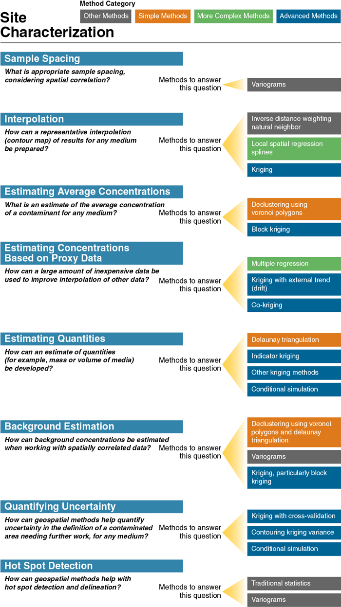
Figure 3. Site characterization overview.

Site Characterization: Sample Spacing

What is appropriate sample spacing, considering spatial correlation?

▼Read more

Choosing efficient and effective sample spacing (in space or time) for any medium can help to optimize a sampling program. For any site, the applicable environmental media may vary and evaluations may be conducted for multiple environmental media. The purpose for each evaluation may differ by medium as well; see Common Misapplications for information on how these differences can result in misapplication of geospatial methods. Additionally, see the discussion on using geospatial results in selection of sample spacing or sampling plan design.

Geospatial Method:

Variograms (spatial or temporal) can identify distances in space or time where samples would provide independent (noncorrelated) data so that the effort does not yield duplicative information. The range interpreted from the variogram is an indication of the spacing of noncorrelated data. A large fraction of the range is a reasonable basis for sample spacing.

Site Characterization: Interpolation

How can a representative interpolation (contour map) of results for any medium be prepared?

▼Read more

A representative map that effectively portrays the spatial relationships of sampling and measurement results supports optimal site decisions.

Geospatial Methods:

  1. Simple geospatial methods such as inverse distance weighting or natural neighbor interpolation
  2. More complex geospatial methods such as local spatial regression or splines
  3. Advanced methods (kriging)

Site Characterization: Estimating Average Concentrations

What is an estimate of the average concentration of a contaminant for any medium?

▼Read more

For treatment design, risk assessment, and other objectives it may be necessary to estimate the average for potentially correlated spatial data. If data are spatially correlated or clustered, geospatial methods may yield more accurate estimates of the average. Another approach to find average concentrations would be to conduct incremental sampling, which provides a physical average (see ITRC ISM-1). For more information, see the discussion of using geospatial results in estimating quantities and average concentrations.

Geospatial Methods:

  1. Declustering using Voronoi polygons with values weighted by area of polygons
  2. Block kriging to estimate the average concentration in a specific area or block, particularly where data are spatially correlated or clustered.

Site Characterization: Estimating Concentrations Based on Proxy Data

How can a large amount of inexpensive data be used to improve interpolation of other data?

▼Read more

Inexpensive proxy concentrations are often generated by other means such as real-time field measurements and can be correlated with fewer fixed laboratory data points, can be used together to make better site characterization maps. This method can be used with the Triad approach (ITRC 2003; ITRC 2007; USEPA 2003). For more information, see the discussion of using geospatial results in using proxy information to estimate contaminant concentrations.

Geospatial Methods:

  1. Multiple regression
  2. Kriging with external trend (drift)
  3. Co-kriging

Site Characterization: Estimating Quantities

How can an estimate of quantities (for example, mass or volume of media) be developed?

▼Read more

Geospatial analysis can help to optimize the estimate of quantities needing remediation and quantify the uncertainty associated with that estimate. The answer to this question also determines the limits of the media that require treatment. This approach can also be useful for risk assessment and remedial design; see also the discussion of using geospatial results in estimating quantities.

Geospatial Methods:

  1. Delaunay triangulation can be used to estimate the areas of exceedance.
  2. Indicator kriging provides certainty of exceedances of the standard to assess risk and cost tradeoffs, which is particularly useful for remedial design.
  3. Other kriging methods can be used to interpolate between known values to assess limits and uncertainties with kriging variances.
  4. Conditional simulation can be conducted to assess the probabilities of volumes or areas exceeding a standard.

Site Characterization: Background Estimation

How can background concentrations be estimated when working with spatially correlated data?

▼Read more

Sampling results that are clustered and spatially correlated can skew the background statistics. Geospatial methods address this problem by better representing background concentrations that vary spatially. The products of the analysis can be measurements of spatial correlations of existing data, as well as an estimate of the true background population statistical distribution when working with spatially correlated data. For more information, see the discussion of using geospatial results in background estimation.

Geospatial Methods:

  1. Declustering using Voronoi polygons and Delaunay triangulation, with values weighted by area of polygons.
  2. Variograms (for assessing if the data are spatially correlated).
  3. Kriging, particularly block kriging where background data are spatially correlated or clustered.

Site Characterization: Quantifying Uncertainty

How can geospatial methods help quantify uncertainty in the definition of a contaminated area needing further work, for any medium?

▼Read more

Analysis of uncertainty when contouring environmental data may help inform and optimize the decisions about future sampling locations or areas requiring remediation (for example excavation quantity or spatial extent). The analysis provides maps of uncertainty in the estimated or interpolated values. For more information, see the discussion of using geospatial results in quantifying uncertainty.

Geospatial Methods

  1. Kriging (various types) with cross-validation, and contouring kriging variance in order to look for areas of high variance as areas of uncertainty
  2. Contouring kriging variance, looking for areas of high variance as areas of uncertainty
  3. Conditional simulation can be used to assess how the interpolated or predicted values may vary over many realizations. This approach can provide values of probabilities for exceedances.

Site Characterization: Hot Spot Detection

How can geospatial methods help with hot spot detection and delineation?

▼Read more

During regular monitoring or characterization, it is important to delineate localized but very strong contaminant source areas (hot spots). These areas can be identified by sampling on a systematic grid or through use of row- and column-aligned incremental sampling methods (ISM). Traditional statistical analysis can help identify a strategy to find hot spots, but does not take into account any spatial correlation over short distances. Geospatial analysis of data may help identify these hot spots. Examples of geospatial analysis approach include ordnance detection with geophysical data, or characterization of a large area with random storage or disposal of hazardous wastes. Note that geospatial methods require some existing data to guide the collection of additional data. For more information, see the discussion of using geospatial results in Hot Spot Detection/Delineation.

Geospatial Methods:

  1. Variograms can help select optimal grid spacing based on the degree of spatial correlation for detecting hotspots of a given size. The variograms can indicate the distances at which the sampling locations can be spaced without too much duplicative information. Hot spots usually have high variability over short distances, so closer spacing is appropriate.

image_pdfPrint this page/section


GRO

web document
glossaryGRO Glossary
referencesGRO References
acronymsGRO Acronyms
ITRC
Contact Us
About ITRC
Visit ITRC
social media iconsClick here to visit ITRC on FacebookClick here to visit ITRC on TwitterClick here to visit ITRC on LinkedInITRC on Social Media
about_itrc
Permission is granted to refer to or quote from this publication with the customary acknowledgment of the source (see suggested citation and disclaimer). This web site is owned by ITRC • 1250 H Street, NW • Suite 850 • Washington, DC 20005 • (202) 266-4933 • Email: [email protected] • Terms of Service, Privacy Policy, and Usage Policy ITRC is sponsored by the Environmental Council of the States.