Build Geospatial Model
Once a general geospatial method has been selected, the data and CSM are used to select appropriate values for the parameters that are relevant for that method. The detailed method descriptions include the parameters that must be selected for each method. Generally, an iterative process is used to build a geospatial model. Based on an initial model, geospatial results are generated and mapped, and then the model is evaluated for accuracy and consistency with the CSM. Typically, alternative models with different parameter values are also constructed and the accuracy of the results from different models are compared using cross-validation. Often, many different models have similar cross-validation performance. In general, use the model with the fewest parameters that has good cross-validation performance.
The goal of the model is to reproduce the variation in the data. In general, geospatial models can have three components: trend (large-scale variation), spatial correlation (small-scale variation), and error. The error component includes both measurement error and variation occurring on a scale smaller than the sample spacing. The first choice to make when selecting a model is whether it is necessary to model uncertainty in the results. If the main purpose is mapping, then there may be no need to put the effort into carefully modeling the spatial correlation or error components. A simple method (or any method with default parameters) can be used with adjustments to the method parameters made to produce a set of predictions that are visually appealing and consistent with the CSM.
If it is important to quantify uncertainty in the prediction, then use a more complex or advanced method. More complex methods (and also simple methods) represent all of the pattern in the data using the trend component. This practice works best when there are other explanatory variables available that are correlated with the primary variable of interest. Ideally, the trend component captures all of the important variation so that the residuals from the trend model have no remaining spatial correlation. If there is significant spatial correlation in the trend residuals, an advanced method is needed so that a spatial correlation component can be included in the model.
If an advanced method is used, then the standard approach is to a use a relatively simple model for the trend, based on a low-order polynomial regression on the coordinates. In some cases, a more detailed model of the trend using local or multiple regression may give better results. The trend model should ideally have a physical basis, such as distance to a contamination source. A good trend model is particularly important if the model is used to extrapolate beyond the area of existing data.
The effect of the choice of trend model can be evaluated using cross-validation. The residuals after removing the trend from the data should be approximately stationary, in order to allow the spatial correlation model to be estimated from the data. Stationarity means that the statistical properties (such as spatial correlation) are the same in different locations. This requirement allows data from different locations to be combined to estimate the spatial correlation model that is applicable throughout the area sampled.
In addition to detrending, the data may also need to be transformed to be normally distributed. An assumption of normality is required in order to quantitatively use the estimates of prediction uncertainty. Otherwise, the uncertainty estimates can only be used in a relative sense to determine where the prediction uncertainty is larger and where it is smaller.
After detrending and transformation, the data can be used to model spatial correlation. The spatial correlation component of the model consists of a variogram (or covariogram) model that is fit to the transformed or detrended data. The process for fitting a variogram model to the empirical variogram is as follows:
- Choose a suitable variogram model, with or without a nugget.
- Fit the model by eye or with software.
- Examine the resulting fit visually and using cross-validation.
Another modeling decision is the choice of search neighborhood. The search neighborhood determines how many nearby points will be used for prediction at each location. There are several reasons for limiting the number of points used through a search neighborhood. First, if there are more than several hundred data points, it may be computationally infeasible to use all of the data. Second, due to uncertainties in the variogram model at larger lag distances, a smaller search neighborhood may give more accurate predictions than a larger search neighborhood. Finally, using a search neighborhood makes the assumption of stationarity much easier to meet, since only each local neighborhood needs to be stationary instead of the entire data domain. As with all modeling choices, model cross-validation can assist with determining the best approach.
Example
To illustrate the model building work flow, consider an alternative approach to modeling the Meuse River zinc data. For this example, instead of using nonparametric regression, other methods can be used to achieve similar results. The zinc concentration data are skewed, so the process begins by log transforming the data to make it more normally distributed. The empirical variogram of the log-transformed data is shown in Figure 42. Potential theoretical variogram models are selected based on an examination of the empirical variogram. The spherical and exponential models are reasonable candidates because they have a similar shape to the empirical variogram. These two models were fit to the empirical variogram using software, with the resulting fits shown in Figures 43 and 44.
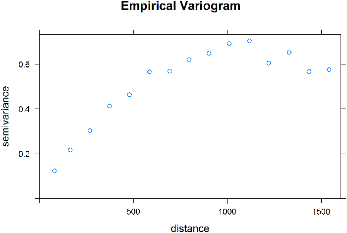
Figure 42. Empirical variogram of log zinc concentrations.
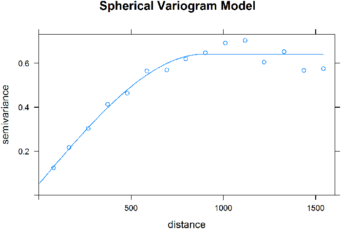
Figure 43. Spherical variogram model fit.
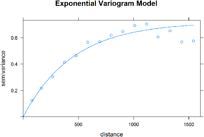
Figure 44. Exponential variogram model fit.
The EDA conducted in the regression example shows that the zinc concentration is correlated with distance from the river. There is a linear relationship between log zinc concentration and the square root of distance from the river. An alternative trend model can next be developed based on a regression on the square root of distance. After fitting this trend model, a variogram of the residuals is fit using a spherical model as shown in Figure 45.
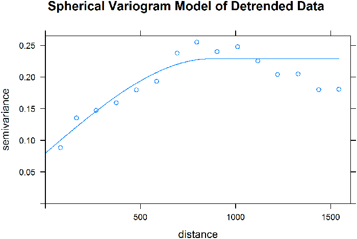
Figure 45. Spherical variogram fit to detrended data.
Visually, these variogram models all appear to fit the data well. What if the predictions from these variogram models were based on kriging instead? Or an interpolation using IDW? Figure 46 shows the predictions for log zinc for the four approaches: (1) IDW; (2) ordinary kriging (OK) with the spherical variogram; (3) OK with the exponential variogram; and (4) kriging with external drift (KED), kriging with external trend, with the spherical variogram. Ordinary kriging uses a constant for the trend component (no trend), while kriging with external drift is using the regression based on distance to the river for the trend component. The kriging predictions resemble each other and are much smoother than IDW. In the next section, cross-validation is used to quantitatively evaluate the quality of these fits.
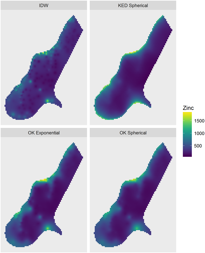
Figure 46. Predictions from four models.

