• Skip to main content
itrc_logo

Geospatial Analysis for Optimization at Environmental Sites

Home
About ITRC
Navigating this Website
Overview
Fact Sheets
Fact Sheets Overview
Fact Sheet 1: Do You Need Geospatial Analysis?
Fact Sheet 2: Are Conditions Suitable for Geospatial Analysis?
Fact Sheet 3: How is Geospatial Analysis Applied?
Fact Sheet 4: What Software is Available to Help?
PM's Tool Box
PM's Tool Box Overview
Review Checklist
Choosing Methods
Common Misapplications
Optimization Questions
Geospatial Analysis Support for Optimization Questions in the Project Life Cycle
Data Requirements
General Considerations
Methods for Optimization
Geospatial Methods for Optimization Questions in the Project Life Cycle Stages
Release Detection
Site Characterization
Remediation
Monitoring
Closure
Documenting Results
Fundamental Concepts
Fundamental Concepts for Geospatial Analysis
Basic Data Concepts for Geospatial Analysis
Interpolation Methods and Model Prediction
Uncertainty in Geospatial Analyses
Characteristics of Interpolation Methods
Work Flow
Work Flow for Conducting Geospatial Analysis
Geospatial Analysis Work Flow Overview
Perform Exploratory Data Analysis
Select Geospatial Method
Build Geospatial Model
Evaluate Geospatial Method Accuracy
Generate Geospatial Analysis Results
Using Results
Using Analysis Results for Optimization
Plume Intensity and Extent
Trend Maps
Estimating Quantities
Hot Spot Detection
Sample Spacing
Estimating Concentrations Based on Proxy Data
Background Estimation
Quantifying Uncertainty
Remedial Action Optimization
Monitoring Program Optimization
Examples
Examples Overview
Example 1
Example 2
Example 3
Example 4
Methods
Methods Overview
Simple Geospatial Methods
More Complex Geospatial Methods
Advanced Methods
Index of Methods
Software
Software Overview
Software Comparison Tables
Software Descriptions
Workshops and Short Courses
Case Studies
Case Studies Overview
Superfund Site Monitoring Optimization (MAROS)
PAH Contamination in Sediments—Uncertainty Analysis (Isatis)
Optimization of Long-Term Monitoring at Former Nebraska Ordnance Plant (GTS; Summit Envirosolutions)
Optimization of Lead-Contaminated Soil Remediation at a Former Lead Smelter (EVS/MVS)
Extent of Radiological Contamination in Soil at Four Sites near the Fukushima Daiichi Power Plant, Japan (ArcGIS)
Optimization of Groundwater Monitoring at a Research Facility in New Jersey (GWSDAT)
Optimization of Sediment Sampling at a Tidally Influenced Site (ArcGIS)
Stringfellow Superfund Site Monitoring Optimization (MAROS)
Lead Contamination in Soil (ArcGIS)
Stakeholder Perspectives
Additional Information
Project Life Cycle Stages
History of Remedial Process Optimization
Additional Resources
Acronyms
Glossary
Index of Methods
Acknowledgments
Team Contacts
Document Feedback


Geospatial Analysis for Optimization at Environmental Sites
HOME

Example 2

Example 2: Plume Shrinkage Analysis
Application: Plume shrinkage analysis
Application Summary: Plume concentrations were interpolated over different time steps during in-situ remediation to quantify trends in mass reduction.
Software: Surfer, ArcGIS or other software capable of spatial interpolation and grid math or area/volume analysis.
Methods: Any interpolation method, grid multiplication, or grid volume and area calculations.
Data Requirements: See recommendations regarding data requirements for kriging.
Reference: Ricker 2008
Approach: Plume shrinkage over time is an important remediation question identified in Section 2. Evaluating this question involves creating a series of geostatistical plume maps at distinct times to assess reductions in extent and/or intensity. Changes in plume area, average concentration, and mass over time can be quantified using grid or raster tools in software such as Surfer or ArcGIS. These metrics can then be statistically trended to evaluate remedial progress and inform optimization decisions. This process is similar to spatial moment analysis as performed in MAROS, but allows more flexibility as plume mass calculations are performed manually by the user using any interpolation method.


Results: Figure 54 is an example, hypothetical visualization showing reductions in plume size and total dissolved phase mass during in-situ remediation. These plume maps and mass calculations were performed in ArcGIS through the following steps:
  • Interpolate monitoring well concentrations and aquifer saturated thickness measurements using kriging or another method to create raster grids of continuous predictions.
  • Convert these floating point rasters to integer rasters.
  • Convert the integer rasters to polygons and join concentration and thickness properties together in the same feature class using a union command.
  • Calculate the area of each grid cell using the calculate geometry function.
  • Calculate the dissolved mass of each cell by multiplying the area by the saturated thickness by the concentration by the porosity (which could be an assumed uniform value or an interpolated grid like saturated thickness).

Ricker (2008) describes an alternative approach to calculating plume mass using Surfer. After creating an interpolated concentration grid in Surfer, a grid volume report can be generated to calculate the positive volume and planar area of the grid. The average plume concentration can be approximated as the concentration grid volume (in units of µg/L*m2) divided by the concentration grid planar area. The plume boundary concentration representing the outer extent of the planar area should be added to the calculated average concentration. To obtain mass, this average concentration can be multiplied by the plume area and assumed uniform values of saturated thickness and porosity.

gro_fig_9_5

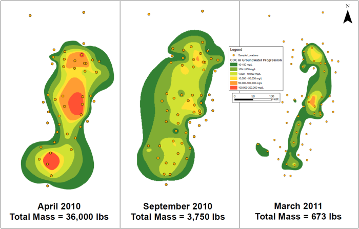
Figure 54. Plume shrinkage and mass reduction over time.
Source: Courtesy of Ted Parks, AMEC Foster Wheeler.

image_pdfPrint this page/section


GRO

web document
glossaryGRO Glossary
referencesGRO References
acronymsGRO Acronyms
ITRC
Contact Us
About ITRC
Visit ITRC
social media iconsClick here to visit ITRC on FacebookClick here to visit ITRC on TwitterClick here to visit ITRC on LinkedInITRC on Social Media
about_itrc
Permission is granted to refer to or quote from this publication with the customary acknowledgment of the source (see suggested citation and disclaimer). This web site is owned by ITRC • 1250 H Street, NW • Suite 850 • Washington, DC 20005 • (202) 266-4933 • Email: [email protected] • Terms of Service, Privacy Policy, and Usage Policy ITRC is sponsored by the Environmental Council of the States.