PAH Contamination in Sediments—Uncertainty Analysis (Isatis)
Contact: Gael Plassart, ENVISOL, mailto:[email protected]
Problem Statement
Sediments have been affected because of the loading and unloading of goods carried on boats arriving at the dock in Gaspé Bay harbor. The contamination is likely to migrate from the dock to Gaspé Bay.
Site Background
Gaspé Bay harbor has operated since the beginning of the twentieth century and has had several uses including military, industrial, and commercial.
Several characterization investigations have been performed at the site since 1998. These studies have revealed PAH contamination in sediments that extends from the dock to the Gaspé Bay. In 2011, an additional investigation was conducted throughout the site and consisted of drilling 129 boreholes located in a regular mesh pattern. A first estimate of contaminated sediments was calculated by performing the Thiessen Polygons method. The total volume of contaminated sediments was estimated to be 26,900 m3.
Project Objectives
The goal of the study was to delineate the extent of PAH contamination in sediments and to analyze the uncertainties of the estimates by using geospatial methods. The results were then compared to the initial estimates calculated with the Thiessen Polygons method.
Data Set

This study evaluates the data set obtained during the characterization investigation conducted in 2011. In total, 377 samples, collected at a rate of two to three per borehole, were analyzed in the laboratory. Samples were collected between 30 cm and 90 cm in depth. Minimal sampling was performed in the northwest area, and no sampling was performed in the south and east areas, at depths between 60 cm and 90 cm.
Methods
The steps of the study were conducted as follows:
- EDA
- Construction of the empirical variogram and fitting
- Conditional simulation
EDA
EDA was performed in order to visualize general trends and possible anisotropies. The first results highlighted three important points:
- Deep sampling was not performed at the South and the East part of the site between 60 cm and 90 cm depth (see Figure 85).
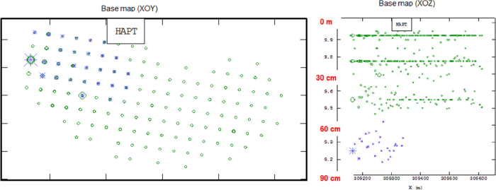 Figure 85. Sample locations (samples collected from 60 cm to 90 cm depth).
- The variogram map showed a possible anisotropy following the N110° (Figure 86). An important question was: is this anisotropy associated with the behavior of the contamination in the sediments or does it correspond to a preferential direction of sampling?
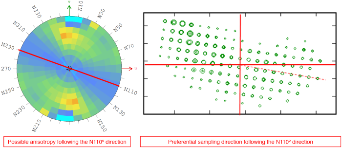 Figure 86. Variogram map.
- The distribution of the contaminants showed a skewed histogram (Figure 87).
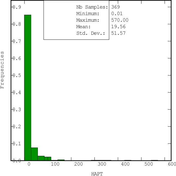 Figure 87. Histogram.
Construction of the Empirical Variogram and Fitting
According to the observations revealed by the EDA, several empirical variograms and models were constructed in order to verify whether the anisotropy was intrinsically associated with the contamination’s behavior or if it corresponded to a sampling effect. The cross-validation revealed that the best variogram and model corresponded to the isotropic model (see Figure 88).
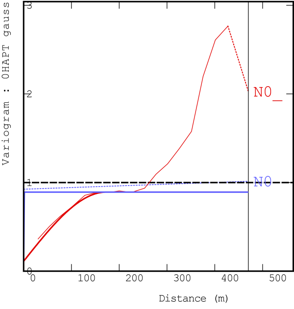 Figure 88. Final variogram using Gaussian-transformed data.
The final variogram was constructed with the Gaussian-transformed data because the conditional simulation method requires this type of transformation.
Conditional Simulation Method
To achieve mapping of contaminated areas and to estimate the volume of contaminated sediments, the conditional simulation were chosen because:
- The histogram of original data showed a skewed distribution. In these cases, the mean of the distribution is not representative of the data set. Using the kriging method can introduce some bias because it performs the estimates of concentrations by using local means.
- The conditional simulation method allows to identify and quantify the uncertain volumes.
Figure 89 illustrates the probabilities of exceeding the remediation threshold of 5 ppm set for the PAHs. This chart represents the sediments showing a probability to be contaminated of 30% or more. This 3D map takes into account the contamination sources (high risk of contamination > 60%) and the uncertain areas (30–60%). Furthermore, the map illustrates the most probable volume predicted by the conditional simulation method (median of the risk curve).
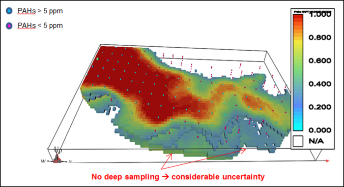 Figure 89. Probabilities of exceeding the remediation threshold of 5 ppm for PAH measurements.
The areas of uncertainty are mainly located at the southeast part of the site, where a deep sampling was not performed.
The estimate volume of contaminated sediments, 43,440 m3, was calculated using the conditional simulation and is shown in Figure 90. The uncertain volume is 14,500 m3.
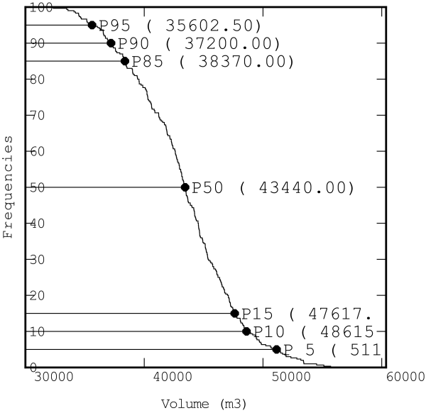 Figure 90. Estimated volume of contaminated sediments.
Results
The volume of contaminated sediments obtained by the Thiessen polygons method was estimated to be 26,900 m3. Comparing this result to the estimate performed by the conditional simulation, the volumes are similar without taking into account the uncertain volume (see Table 11).
Table 11. Comparison of estimated volumes using Thiessen polygons and conditional simulation
| Comparison of estimated volumes by performing different methods | |
|---|---|
| Estimated volume of contaminated sediments by performing geostatistics | 43,440 m3 |
| Uncertain volume | 14,500 m3 |
| Estimated volume of contaminated sediments by performing polygons | 26,900 m3 |
The areas that have not been sampled have not been taken into account for the estimates of contaminated sediments. The lack of analysis, however, does not imply the absence of contamination.
Outcome
Missing the uncertainties associated with each stage of a characterization project may lead to unreliable estimates of contamination. The quantification and localization of uncertain areas allow accurate assessment of the financial risk of the project and, if needed, definition of a complementary sampling characterization appropriate for each area.

