• Skip to main content
itrc_logo

Geospatial Analysis for Optimization at Environmental Sites

Navigating this Website
Overview
Fact Sheets
Fact Sheets Overview
Fact Sheet 1: Do You Need Geospatial Analysis?
Fact Sheet 2: Are Conditions Suitable for Geospatial Analysis?
Fact Sheet 3: How is Geospatial Analysis Applied?
Fact Sheet 4: What Software is Available to Help?
PM's Tool Box
PM's Tool Box Overview
Review Checklist
Choosing Methods
Common Misapplications
Optimization Questions
Geospatial Analysis Support for Optimization Questions in the Project Life Cycle
Data Requirements
General Considerations
Methods for Optimization
Geospatial Methods for Optimization Questions in the Project Life Cycle Stages
Release Detection
Site Characterization
Remediation
Monitoring
Closure
Documenting Results
Fundamental Concepts
Fundamental Concepts for Geospatial Analysis
Basic Data Concepts for Geospatial Analysis
Interpolation Methods and Model Prediction
Uncertainty in Geospatial Analyses
Characteristics of Interpolation Methods
Work Flow
Work Flow for Conducting Geospatial Analysis
Geospatial Analysis Work Flow Overview
Perform Exploratory Data Analysis
Select Geospatial Method
Build Geospatial Model
Evaluate Geospatial Method Accuracy
Generate Geospatial Analysis Results
Using Results
Using Analysis Results for Optimization
Plume Intensity and Extent
Trend Maps
Estimating Quantities
Hot Spot Detection
Sample Spacing
Estimating Concentrations Based on Proxy Data
Background Estimation
Quantifying Uncertainty
Remedial Action Optimization
Monitoring Program Optimization
Examples
Examples Overview
Example 1
Example 2
Example 3
Example 4
Methods
Methods Overview
Simple Geospatial Methods
More Complex Geospatial Methods
Advanced Methods
Index of Methods
Software
Software Overview
Software Comparison Tables
Software Descriptions
Workshops and Short Courses
Case Studies
Case Studies Overview
Superfund Site Monitoring Optimization (MAROS)
PAH Contamination in Sediments—Uncertainty Analysis (Isatis)
Optimization of Long-Term Monitoring at Former Nebraska Ordnance Plant (GTS; Summit Envirosolutions)
Optimization of Lead-Contaminated Soil Remediation at a Former Lead Smelter (EVS/MVS)
Extent of Radiological Contamination in Soil at Four Sites near the Fukushima Daiichi Power Plant, Japan (ArcGIS)
Optimization of Groundwater Monitoring at a Research Facility in New Jersey (GWSDAT)
Optimization of Sediment Sampling at a Tidally Influenced Site (ArcGIS)
Stringfellow Superfund Site Monitoring Optimization (MAROS)
Lead Contamination in Soil (ArcGIS)
Stakeholder Perspectives
Additional Information
Project Life Cycle Stages
History of Remedial Process Optimization
Additional Resources
Acronyms
Glossary
Index of Methods
Acknowledgments
Team Contacts
Document Feedback


Geospatial Analysis for Optimization at Environmental Sites
HOME

Evaluate Geospatial Method Accuracy

Before using the predictions or prediction uncertainty estimates, the overall accuracy of the interpolation method or model must be assessed. The interpolated values should be checked to make sure they are consistent with the CSM and other source of information. In addition, the method should be evaluated using formal statistical methods for assessing model fit. The primary model assessment methods are cross-validation and validation.
▼Read more

Cross-validation involves eliminating one observed value at a time from the data set, using the model to calculate a predicted value at that point, and then comparing the predicted value with the observed value. Therefore, if you have N data points, you generate N tests of the validity of the model and this provides an evaluation of the accuracy of the model. Similarly, a model can be validated by dividing the observed data set randomly into two data sets, and then using each set to calculate predicted values for the other set; this is called two-fold cross-validation. Measures of model accuracy can also be compared to each other in order to select among alternative models. In general, the simplest model with adequate accuracy should be selected for use in the application.

All of the interpolation methods (simple, more complex, and advanced) provide a set of predictions at unsampled locations. More complex and advanced geospatial interpolation methods also provide an assessment of prediction uncertainty at unsampled locations through the prediction of standard error. Conditional simulation provides a more complete characterization of uncertainty because it generates an estimate of the possible distribution of values that might be found at each unsampled location. The predictions and prediction uncertainty measures provided by the geospatial interpolation methods are only accurate if the interpolation method is based on a model that adequately fits that data.

Cross-Validation

▼Read more

The most common way to evaluate model accuracy or quality of fit is through cross-validation. Cross-validation allows assessment of the accuracy of an interpolation model by computing and investigating the prediction errors, also referred to as residual errors (or “residuals”). The residual errors are calculated by removing the first observation from the data set, and using the remaining data and the specified model to predict a value at that location. The difference between the data value and the predicted value is the residual:

Residual error = interpolated value − observed value

This process is repeated for each individual data value and summary statistics are then calculated for the residual data set (Golden Software 2002). This is sometimes referred to as “leave-one-out” cross-validation. Other less common methods are the holdout method or k-fold cross-validation, which are not covered in this document.

Validation

▼Read more

Validation entails calculating residuals for measurement locations that were not used in the original interpolation. The data are randomly divided into two groups: the test data set and the training data set. The training data set is used to develop the model and make predictions at the locations of the test data set. Residuals are calculated at the test data locations. Validation is generally a better way to assess prediction accuracy than cross-validation because it does not use any of the data from the original interpolation model, reducing the associated bias that makes the model appear to perform better than it does in reality.

Different sets of cross-validation and validation statistics are available for performing model diagnostics depending on the complexity of the model used. This method is further described in the sections below.

Determine Errors in Simple Methods

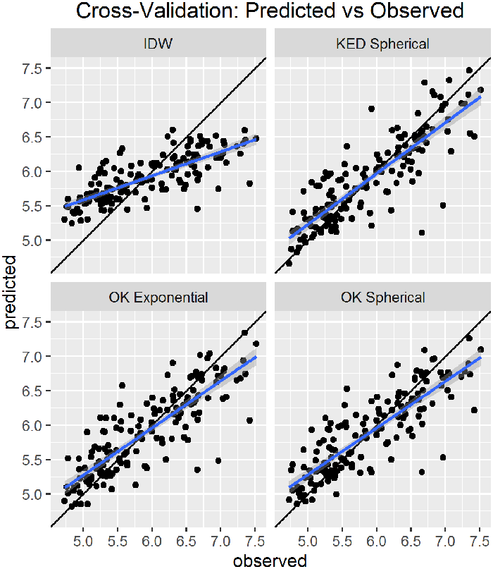
For simple geospatial models (for example, IDW), after computing the cross-validation or validation errors, the mean error (same units as the data, measuring the prediction bias) and the root-mean-square error (RMSE, measuring prediction accuracy) can be calculated. Simple methods do not estimate prediction uncertainty across sample locations; however, cross-validation may be used to estimate variation at individual sample locations.

▼Read more

Other statistics such as the absolute residual mean (mean of absolute value residuals), residual standard deviation, or scaled RMSE (RMSE divided by range of the data) may be helpful in the analysis. It is standard practice to plot the predicted values versus the measured values, and the residual values versus the measured values to help reconcile the calculated statistics. It is also useful to plot the residuals on a map and interpolate them to produce a continuous surface of interpolation error. This approach helps to assess whether the interpolation model performs better or worse in certain portions of the site.

When interpreting the cross-validation/validation statistics for simple geospatial models, consider the following factors (Johnston et al. 2003):

  • Predictions should be as close to the measurement values as possible, that is, the scatter along the straight line on the graphs should be minimal; the smaller the root-mean-square prediction error, the better.
  • Predictions should be unbiased (centered on the measurement values). If the prediction errors are unbiased, then the mean prediction error should be near zero without a significant positive or negative bias.

Acceptable cross-validation/validation error thresholds are project specific and should be made based on interpolation objectives and considering the scale of the data. These statistics are most useful in comparing the performance of different interpolation models to help select the most accurate one.

Determine Errors in More Complex and Advanced Methods

In addition to predictions at unsampled locations, more complex (regression) and advanced (geostatistical) methods also provide the prediction standard errors that provide an estimate of uncertainty at each prediction location. Three additional metrics of method accuracy can be calculated: mean standardized error (dimensionless), average standard error (analogous to root mean square error), and root-mean-square standardized error (measuring the assessment of prediction variability). Beyond assessing the overall ability of the model to make good predictions, this additional set of statistics allows assessment of how accurately the model reflects the variability of the data. The mean error and RMSE are still useful metrics for advanced methods and should be calculated and presented as with simple methods.

▼Read more

When interpreting the cross-validation/validation statistics for regression and geostatistical models, consider the following factors (Johnston et al. 2003):

  • Prediction errors depend on the scale and units of the data, so it is better to assess standardized prediction errors, which are given as prediction errors divided by their prediction standard errors. The mean of these should also be near zero.
  • If the average standard error is close to the root-mean-square prediction error, then the model generally reflects the variability of the data, and the root-mean-square standardized error should be close to one. Variability is likely overestimated if the average standard error is greater than the root-mean-square prediction error, or if the root-mean-square standardized error is less than one. Variability is likely underestimated if the average standard error is less than the root-mean-square prediction error, or if the root-mean-square standardized error is greater than one.

When comparing the performance of regression and geostatistical models through cross-validation, the better model will have the standardized mean nearest to zero, the smallest root mean square prediction error, the average standard error nearest the root mean square prediction error, and the standardized root mean square prediction error nearest to one. For regression methods, other goodness-of-fit criteria, such as the Akaike information criterion (AIC) and the Bayesian information criterion (BIC), can also be used to support the choice of model and goodness-of-fit assessment (Akaike 1974; Sakamoto, Ishiguro, and Kitagawa 1986).

Examples

▼Read more

Cross-validation was used to evaluate the four models displayed in Figure 46. One way to graphically evaluate the results is to plot the predicted value versus the observed value, as shown in Figure 47. If the predictions match perfectly, the points plot on a diagonal line. The best fit line to the points is shown on the figure in blue. The fit lines for all four of the models have a flatter slope than the 45-degree line show in black. All of the methods tend to smooth the data, leading to underprediction of the higher values and overprediction of the lower values. This is a general characteristic of all interpolation methods except conditional simulation.

The cross-validation statistics for the four models are shown in Table 4. Cross-validation finds the prediction error at each of the data points by comparing the prediction from the model after withholding the data point to the observed value. The prediction error is the difference between the prediction and the observed value. These errors are summarized in two ways: the mean and the root mean square (RMS). The mean error indicates whether the predictions are biased by being on average too high or too low. The RMS error is a measure of the total error in either direction.

Kriging methods also produce a prediction standard error at each location. For these methods, a standardized cross-validation error can be calculated by dividing the cross-validation prediction error by the prediction standard error. If the RMS standardized prediction error is less than one, it means that the method is producing prediction standard errors that overestimate the actual prediction error. If the RMS standardized error is more than one, the method is underestimating the actual prediction errors.

As shown in Table 4, the three kriging methods produce a much lower RMS error than IDW. There is little difference between the performance of the ordinary kriging methods with different variogram models. Ordinary kriging assumes no trend, only a constant mean. Kriging with external drift (trend) models the trend with a regression on distance to the river, resulting in a significant improvement in RMS error. In addition, kriging with external drift has a RMS standardized error closer to one than the ordinary kriging methods. Based on the cross-validation statistics, in this example kriging with external drift yields the best results.

gro_wf_22

Figure 47. Predicted values versus observed values.

Table 4. Cross-validation statistics

Cross-Validation Statistics
Method Variogram Mean Error Root Mean Square Error Mean Standardized Error Root Mean Square Standardized Error
IDW NA -0.0128 0.514 NA NA
Ordinary Kriging Exponential 0.00213 0.393 0.00301 0.93
Ordinary Kriging Spherical -2.06E-05 0.392 0.00017 0.90
Kriging with External Drift Spherical -0.00285 0.375 -0.00377 1.04

image_pdfPrint this page/section


GRO

web document
glossaryGRO Glossary
referencesGRO References
acronymsGRO Acronyms
ITRC
Contact Us
About ITRC
Visit ITRC
social media iconsClick here to visit ITRC on FacebookClick here to visit ITRC on TwitterClick here to visit ITRC on LinkedInITRC on Social Media
about_itrc
Permission is granted to refer to or quote from this publication with the customary acknowledgment of the source (see suggested citation and disclaimer). This web site is owned by ITRC • 1250 H Street, NW • Suite 850 • Washington, DC 20005 • (202) 266-4933 • Email: [email protected] • Terms of Service, Privacy Policy, and Usage Policy ITRC is sponsored by the Environmental Council of the States.