• Skip to main content
itrc_logo

Geospatial Analysis for Optimization at Environmental Sites

Home
About ITRC
Navigating this Website
Overview
Fact Sheets
Fact Sheets Overview
Fact Sheet 1: Do You Need Geospatial Analysis?
Fact Sheet 2: Are Conditions Suitable for Geospatial Analysis?
Fact Sheet 3: How is Geospatial Analysis Applied?
Fact Sheet 4: What Software is Available to Help?
PM's Tool Box
PM's Tool Box Overview
Review Checklist
Choosing Methods
Common Misapplications
Optimization Questions
Geospatial Analysis Support for Optimization Questions in the Project Life Cycle
Data Requirements
General Considerations
Methods for Optimization
Geospatial Methods for Optimization Questions in the Project Life Cycle Stages
Release Detection
Site Characterization
Remediation
Monitoring
Closure
Documenting Results
Fundamental Concepts
Fundamental Concepts for Geospatial Analysis
Basic Data Concepts for Geospatial Analysis
Interpolation Methods and Model Prediction
Uncertainty in Geospatial Analyses
Characteristics of Interpolation Methods
Work Flow
Work Flow for Conducting Geospatial Analysis
Geospatial Analysis Work Flow Overview
Perform Exploratory Data Analysis
Select Geospatial Method
Build Geospatial Model
Evaluate Geospatial Method Accuracy
Generate Geospatial Analysis Results
Using Results
Using Analysis Results for Optimization
Plume Intensity and Extent
Trend Maps
Estimating Quantities
Hot Spot Detection
Sample Spacing
Estimating Concentrations Based on Proxy Data
Background Estimation
Quantifying Uncertainty
Remedial Action Optimization
Monitoring Program Optimization
Examples
Examples Overview
Example 1
Example 2
Example 3
Example 4
Methods
Methods Overview
Simple Geospatial Methods
More Complex Geospatial Methods
Advanced Methods
Index of Methods
Software
Software Overview
Software Comparison Tables
Software Descriptions
Workshops and Short Courses
Case Studies
Case Studies Overview
Superfund Site Monitoring Optimization (MAROS)
PAH Contamination in Sediments—Uncertainty Analysis (Isatis)
Optimization of Long-Term Monitoring at Former Nebraska Ordnance Plant (GTS; Summit Envirosolutions)
Optimization of Lead-Contaminated Soil Remediation at a Former Lead Smelter (EVS/MVS)
Extent of Radiological Contamination in Soil at Four Sites near the Fukushima Daiichi Power Plant, Japan (ArcGIS)
Optimization of Groundwater Monitoring at a Research Facility in New Jersey (GWSDAT)
Optimization of Sediment Sampling at a Tidally Influenced Site (ArcGIS)
Stringfellow Superfund Site Monitoring Optimization (MAROS)
Lead Contamination in Soil (ArcGIS)
Stakeholder Perspectives
Additional Information
Project Life Cycle Stages
History of Remedial Process Optimization
Additional Resources
Acronyms
Glossary
Index of Methods
Acknowledgments
Team Contacts
Document Feedback


Geospatial Analysis for Optimization at Environmental Sites
HOME

Remediation

The goal of the remediation stage is the selection, implementation and operation of actions to prevent exposures and achieve the regulatory limits or cleanup goals where practicable.

Geospatial methods can support and optimize remedy selection and evaluation of remedy effectiveness by:

  • informing the CSM (remedy selection is based on the CSM)
  • assessing the certainty in the required remedial footprint
  • determining the contaminant mass (and its uncertainty) which may support selection, design, and cost estimating of a particular remedy
  • determining the contaminant mass discharge or flux from discrete measurement points before and after treatment. Geospatial methods can provide a better indication of the uncertainty in the mass discharge estimates than other interpolation techniques (Li, Goovaerts, and Abriola 2007); see also the ITRC MASSFLUX-1 document.
  • illustrating the spatial variation which may influence how remedial alternatives are applied
  • providing input to various models intended to simulate and optimize remedial processes
  • evaluating dynamics such as seasonal variation, geochemical changes, and groundwater flow regimes
  • supporting determination of remedy effectiveness and monitoring effectiveness of remedial measures
  • allowing forecasts of remedial duration for attenuation based on spatial and temporal trends
  • supporting predictions of short and long-term remedial effectiveness
  • developing visual description
  • predicting concentrations that are consistent with simulations
  • comparing the results with the bounds of anticipated uncertainty

Figure 4 provides an overview of the role of geospatial methods in this stage of the project life cycle. Each general topic, specific question, and method is linked to a more detailed discussion.

Figure 4 Remediation Overview

Click Here to go to Plume Change/Attenuation Over Time Click Here to go to Trend Maps Click Here to go to Estimating Average Concentration Click Here to go to Evaluating Remedial Success Click Here to go to Remedial Action Optimization Click Here to go to Future Data Prediction/Verification

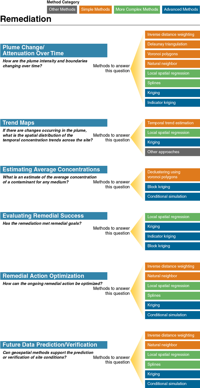
Figure 4. Remediation overview.

Remediation: Plume Change/Attenuation Over Time

How are the plume intensity and boundaries changing over time?

▼Read more

Changes in concentrations over time are key metrics for remediation progress. These changes can be assessed at individual sampling locations, but the plume as a whole cannot be tracked without spatial mapping of the plume at a series of points through time. A series of geospatially interpolated plume maps at distinct times can be compared to assess reductions in extent or intensity, or both. For more information, see the discussion of using geospatial results in plume change over time and estimating quantities, as well as an example of plume shrinkage analysis.

Geospatial Methods

  1. Simple geospatial methods, such as inverse distance weighting, Delaunay triangulation with Voronoi polygons and natural neighbor interpolation on mutually exclusive subsets of the data representing distinct time periods or sampling events can be used to assess plume changes.
  2. More complex geospatial methods, such as local spatial regression or splines.
  3. Advanced methods such as kriging can be used, including indicator kriging with an indicator for the change over time (for example, increasing or decreasing values). Note that indicator kriging can address nondetect concentrations, provided the detection limits are below the concentration goal.

Remediation: Trend Maps

If there are changes occurring in the plume, what is the spatial distribution of the temporal concentration trends across the site?

▼Read more

Geospatial methods can help track plume shrinkage (or expansion) by helping to map the estimated regression slope direction and magnitude of the temporal concentration trends at each sampling location, or the certainty in the direction of the trend for nonparametric methods such as Mann-Kendall analysis. The statistical significance of the trends and the potential for bias in regression results should be considered. The maps can include posted slope values, which can be contoured. Alternatively, the sampling locations can be color-coded based on the direction and magnitude of the trend or the certainty in the direction of the trend. Figure 5 is an example of a trend map for Mann-Kendall trends for benzene concentrations in wells at a site being managed with monitored natural attenuation. A trend map provides a spatial overview of the areas of the site that are decreasing in concentration, as well as how quickly this decrease is occurring; see Trend Maps for a discussion of using geospatial results in understanding the trends.

gro_fig_2_5

Figure 5. Temporal trend map of benzene concentration in wells at monitored natural attenuation site in Texas.
Source: Example trend map courtesy USACE 2015.

Geospatial Methods:

  1. Temporal trend estimation (linear regression, Mann-Kendall, Theil-Sen) can be combined with plotting of the magnitude and direction of the trends on a map. The GSMC-1 document (ITRC 2013) includes more information on trend estimation methods.
  2. More complex methods (for example, local spatial regression) can be used to interpolate the data over both space and time to provide a series of plume maps at different times.
  3. Kriging, including indicator kriging, can be used to map the likely distribution of the determined trend. The statistical confidence in the trend (positive values for increasing trends and negative values for a decreasing trend) can be kriged, or indicator kriging can be used to evaluate certainty of trends by assigning a one to an increasing trend and a zero to the opposite trend.
  4. Other approaches may be used to evaluate changes in plume area, average concentration, and mass over time (quantified using grid or raster tools in software such as Surfer or ArcGIS). These metrics can then be statistically trended to evaluate remedial progress and inform optimization decisions. An example of plume shrinkage analysis illustrates one of these approaches.

Remediation: Estimating Average Concentrations

What is an estimate of the average concentration of a contaminant for any medium?

▼Read more

It is often necessary to estimate the volume or mass requiring cleanup or mass remaining at some point during the remediation. For example, an upper confidence limit on the average concentration may be required to fall below the goal or regulatory threshold; this statistical limit must be estimated with potentially spatially correlated data. Geospatial methods can help in estimating quantities and average concentrations when the data are clustered or spatially correlated.

Geospatial Methods:

  1. Spatial declustering using Voronoi polygons can be used to apply appropriate weights to spatially clustered data in computing an average
  2. Kriging of various kinds can be used to estimate a spatial average with spatially correlated data. This approach includes block kriging to assess averages within specific areas for comparison to a specific goal.
  3. Conditional simulation can be used to assess the likelihood that a site or an area meets or exceeds a specific goal.

Remediation: Evaluating Remedial Success

Has the remediation met remedial goals?

▼Read more

While it may be clear whether individual sampling locations have met remedial goals (see ITRC GSMC-1), it may be important to assess if unsampled locations have also met the goals. This assessment requires a mapping of the site contamination or plume concentrations and comparison to a regulatory or cleanup threshold. Geospatial analysis is most applicable where the goal for an estimate of the average concentration in the environmental medium (for example, soil or groundwater) is to be below a specified criterion over an area. Geospatial methods can also help quantitatively assess the changes in mass flux or discharge as result of cleanup actions (Li, Goovaerts, and Abriola 2007). Output would include maps and measures of uncertainty with the interpolated values. For more information, see the discussion of using geospatial results in evaluating remedial success.

Geospatial Methods:

  1. More complex geospatial methods (for example, local spatial regression) can not only help prepare maps, but also map uncertainty to estimate a confidence envelope around the plume
  2. Advanced methods (kriging) can interpolate concentrations between sampling locations. In particular, indicator kriging can help map probabilities of exceeding or not exceeding the cleanup threshold at any site location. Block kriging can help assess success within an area or total mass flux.

Remediation: Remedial Action Optimization

How can the ongoing remedial action be optimized?

▼Read more

Remedial actions optimization evaluation should always be conducted during remedy implementation. Though optimization of active remedies involves primarily engineering and hydrogeologic analyses, geospatial methods can support these analyses. This support includes preparing current maps of data such as groundwater elevations, contaminant concentrations, in situ treatment amendment concentrations, or geochemical conditions.

Trend maps can help to identify whether areas are responding to treatment as expected. Data generated by sampling during remediation, such as excavation or dredging, can be reassessed to identify additional media requiring removal. If groundwater flow and contaminant modeling is used for optimization evaluation, then geospatial methods can help develop input for the models based on observations. For example, kriging or local spatial regression can be used to interpolate observed values of hydraulic conductivity, water levels, or concentrations for model cells. Conditional simulation can help assess the sensitivity of the modeled, optimized remedy to uncertainty in the interpolated values of the site parameters used in design of the remedy. For more information, see the discussion of using geospatial results in remedial action optimization.

Geospatial Methods:

  1. Simple geospatial methods such as inverse distance weighting, natural neighbor for maps and interpolation.
  2. More complex geospatial methods such as local spatial regression or splines for maps and interpolation.
  3. Kriging for maps and interpolation.
  4. Conditional simulation for assessing model output regarding optimized, modeled remedy.

Remediation: Future Data Prediction/Verification

Can geospatial methods support the prediction or verification of site conditions?

▼Read more

Geospatial methods can provide input for models that allow prediction of future conditions or outcomes, or that can be used to evaluate the optimum design. Geospatial methods can provide an objective way to interpolate values of input parameters for predictive models. Once cleanup targets are initially met, new data may be periodically collected to ensure cleanup goals are maintained and comparison of the new data to previous estimates of concentration distribution may be necessary. Geospatial methods can interpolate new data in map form for comparison to previously prepared predictive maps to detect inconsistencies.

Geospatial Methods:

  1. Simple geospatial methods, including inverse distance weighting, and natural neighbor interpolation can be used to map the data and provide some measure of confidence limits or envelope around the plume. A comparison of each new measurement can be made to see if it falls within the confidence envelope; any measurements outside the envelope are flagged as inconsistent with the remediated plume and require follow-up.
  2. More complex geospatial methods such as local spatial regression and splines can be used in a similar way.
  3. Kriging, of various types, can be used to map the data, including recontouring of the kriging variance with the new data.
  4. Advanced methods such as conditional simulation can be performed. This process could involve including the new data in the sampled distributions to see if the probability of exceeding a specific threshold has changed.

image_pdfPrint this page/section


GRO

web document
glossaryGRO Glossary
referencesGRO References
acronymsGRO Acronyms
ITRC
Contact Us
About ITRC
Visit ITRC
social media iconsClick here to visit ITRC on FacebookClick here to visit ITRC on TwitterClick here to visit ITRC on LinkedInITRC on Social Media
about_itrc
Permission is granted to refer to or quote from this publication with the customary acknowledgment of the source (see suggested citation and disclaimer). This web site is owned by ITRC • 1250 H Street, NW • Suite 850 • Washington, DC 20005 • (202) 266-4933 • Email: [email protected] • Terms of Service, Privacy Policy, and Usage Policy ITRC is sponsored by the Environmental Council of the States.