State Road 114 Superfund Site Monitoring Optimization (MAROS)

Contact: Kirby Biggs, USEPA, [email protected]

Problem Statement

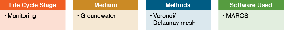
Affected groundwater from a former oil refinery migrated downgradient to private water supply and irrigation wells and threatened municipal water supply wells. Remedial systems have been installed and are operational. The groundwater monitoring network must efficiently provide data to demonstrate protectiveness, monitor plume stability, and document progress toward remedial goals. Groundwater monitoring optimization, including geospatial methods, was conducted to identify a spatially efficient network that minimizes both uncertainty and redundancy.

Site Background

The State Road 114 Groundwater Plume Superfund Site is located one mile west of the City of Levelland in Hockley County, Texas. The site consists of a groundwater plume more than a mile long containing the volatile organic contaminants (VOCs) 1,2-dichloroethane (1,2-DCA) and benzene and metals mobilized due to reducing conditions. The source of the groundwater contamination is a former petroleum products refinery that operated between 1939 and 1954. Environmental contamination of groundwater and soil at the site resulted from the refining operations, associated disposal of wastes, spills, and leaks. Sources of ongoing contamination include a petroleum hydrocarbon layer floating on the water table (light nonaqueous phase liquid [LNAPL]), the soil matrix in the LNAPL smear zone, and a benzene vapor plume in the vadose zone. The groundwater remedy consists of a groundwater extraction and treatment system (pump and treat, P&T) and a soil vapor extraction (SVE) system. The groundwater plume extends downgradient toward private water supply and irrigation wells. Levelland City municipal wells are present downgradient from the edge of the plume.

Affected groundwater is encountered at approximately 140 feet below ground surface (ft bgs) with a saturated interval of approximately 40–80 ft. Because of the depth of the saturated interval, the aquifer has been divided vertically into zones: the shallow zone (upper 10–20 ft of saturated unit), intermediate zone (midpoint in the saturated thickness) and the deep zone (lowest 10–20 ft of saturated unit). The zones are hydraulically connected. For the purpose of statistical and spatial analyses, site groundwater data were divided into one shallow/intermediate zone and the deep zone.

Project Objectives

The primary goals of the long-term monitoring optimization (LTMO) were to improve understanding of the groundwater plume while controlling monitoring cost, confirming protectiveness of the remedy, and demonstrating progress toward remedial goals. The goal of the geospatial analysis was to assess plume stability, and identify concentration uncertainty within the monitoring network. Areas with high concentration uncertainty were recommended for additional monitoring wells or site characterization, while wells in low uncertainty areas were recommended for removal from the routine monitoring program. Assessment of plume stability was used to recommend an appropriate monitoring frequency.

Data Set

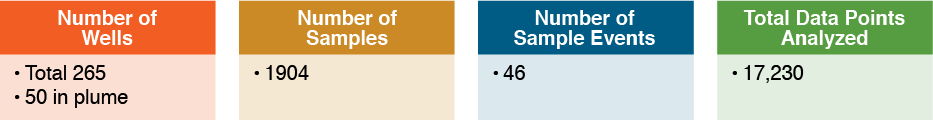
Overall, 265 groundwater monitoring locations have been sampled on site. Many sampling locations are private water supply or irrigation wells. Approximately 26 dedicated groundwater monitoring wells have been installed in the shallow zone, 7 in the Intermediate Zone, and 17 in the deep zone. Monitoring wells of various intervals are organized as nested locations throughout the plumes. Private water supply and irrigation wells are presumed to be screened near the bottom of the saturated zone, and have been sampled to characterize the deep plumes. Samples have been collected from the P&T extraction wells at various times since installation in 2009. The sampling frequency for the network has varied between roughly annual in 2008 and 2009 and semiannual between 2010 and 2012. The number of monitoring, extraction and private supply wells sampled during each sampling event varied between 23 and 51. VOCs constituents are sampled with permeable diffusion bags (PDBs), a method that is not compatible with metals analysis. So, the sampling frequency and, therefore, data set size for metals is less extensive than for VOCs.

Methods

The LTMO analysis was conducted, in part, using methods in the Monitoring and Remediation Optimization System (MAROS) software as well as a qualitative evaluation of site data and the CSM.

The method used to evaluate plume stability includes creation of a Voronoi/Delaunay triangulation mesh for the well network with concentration values for each well node for each sampling event. The mesh is used along with a method of moments approach to estimate the total dissolved contaminant mass, center of mass, and spread of mass in the plume for each sample event. The estimates of mass amount and distribution are then evaluated for trends over time using a Mann-Kendall test for trend. Qualitatively, a decreasing trend for total dissolved mass may indicate that a remedy is performing well. Stable or decreasing trends for plume mass support a decision to reduce monitoring intensity.

Total dissolved mass, center of mass, and spread of mass (zeroth, first, and second moments) were estimated for both benzene and 1,2-DCA plumes in the shallow/intermediate zone. Trends for each moment were evaluated for groundwater data collected from 2008 to 2013, providing metrics for plume stability.

Uncertainty within the network is evaluated using the Voronoi/Delaunay mesh to calculate a slope factor using a natural neighbor approach to compare known concentrations versus estimated concentrations at each location for each sampling event. Locations with high concentration uncertainty are recommended for new well locations, while areas with low concentration uncertainty are recommended for removal from the network. Additional algorithms evaluate if too much information is lost by removing a well location and compare the relative size, concentration magnitude and trends within well areas to prioritize monitoring locations. Areas outside of the current network are identified for new monitoring locations by identifying increasing concentration trends or concentrations above cleanup goals at the down or cross-gradient edges of the network.

Results

The results of the plume stability analysis indicate largely stable trends for plume mass distribution and low to moderate concentration uncertainty between monitoring locations over the time frame of interest. Some limited areas were highlighted, however, for additional delineation or as potential locations for additional wells. An additional nested monitoring location was recommended for the intermediate and deep zones downgradient from the current extent of the monitoring network. Optimally, new wells were recommended at a point on a line between existing locations; roughly two to five years of groundwater travel time downgradient from the existing monitoring locations.

While no other new monitoring locations were recommended, several areas in the shallow/intermediate and deep zones were highlighted as ‘watch’ areas for potential plume migration and increasing concentration uncertainty between monitoring locations. A recommendation was made to reevaluate groundwater data in five years to determine whether additional sampling locations are needed in the watch areas due to plume migration.

One well was identified as a candidate for removal from routine monitoring by the software; however, after qualitative review, the well was recommended for retention in the program to provide vertical information (with nearby nested locations) and data for estimating source mass. Another location (a nondetect upgradient source location) was recommended for removal from the routine monitoring program, to reduce monitoring density in the area. Figure 6-1 shows the results of the calculations.

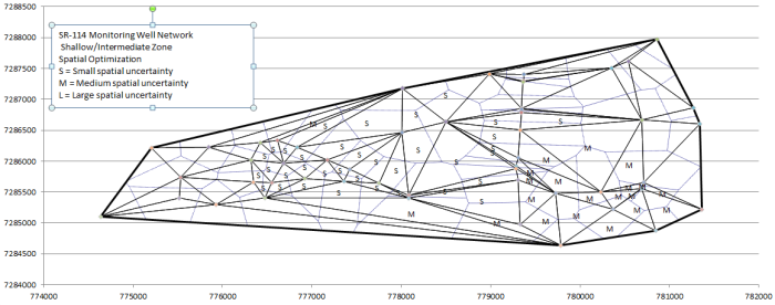
Figure 84. Results for the MAROS calculations for the State Road 114 site.

A total of 83 monitoring locations were identified as providing valuable information addressing site monitoring objectives. Wells in the optimized network were recommended for annual, biennial, or five-year monitoring frequencies based on the magnitude, rate, and trend of contaminant concentration change.

Reference: USEPA 2013b