• Skip to main content
itrc_logo

Geospatial Analysis for Optimization at Environmental Sites

Navigating this Website
Overview
Fact Sheets
Fact Sheets Overview
Fact Sheet 1: Do You Need Geospatial Analysis?
Fact Sheet 2: Are Conditions Suitable for Geospatial Analysis?
Fact Sheet 3: How is Geospatial Analysis Applied?
Fact Sheet 4: What Software is Available to Help?
PM's Tool Box
PM's Tool Box Overview
Review Checklist
Choosing Methods
Common Misapplications
Optimization Questions
Geospatial Analysis Support for Optimization Questions in the Project Life Cycle
Data Requirements
General Considerations
Methods for Optimization
Geospatial Methods for Optimization Questions in the Project Life Cycle Stages
Release Detection
Site Characterization
Remediation
Monitoring
Closure
Documenting Results
Fundamental Concepts
Fundamental Concepts for Geospatial Analysis
Basic Data Concepts for Geospatial Analysis
Interpolation Methods and Model Prediction
Uncertainty in Geospatial Analyses
Characteristics of Interpolation Methods
Work Flow
Work Flow for Conducting Geospatial Analysis
Geospatial Analysis Work Flow Overview
Perform Exploratory Data Analysis
Select Geospatial Method
Build Geospatial Model
Evaluate Geospatial Method Accuracy
Generate Geospatial Analysis Results
Using Results
Using Analysis Results for Optimization
Plume Intensity and Extent
Trend Maps
Estimating Quantities
Hot Spot Detection
Sample Spacing
Estimating Concentrations Based on Proxy Data
Background Estimation
Quantifying Uncertainty
Remedial Action Optimization
Monitoring Program Optimization
Examples
Examples Overview
Example 1
Example 2
Example 3
Example 4
Methods
Methods Overview
Simple Geospatial Methods
More Complex Geospatial Methods
Advanced Methods
Index of Methods
Software
Software Overview
Software Comparison Tables
Software Descriptions
Workshops and Short Courses
Case Studies
Case Studies Overview
Superfund Site Monitoring Optimization (MAROS)
PAH Contamination in Sediments—Uncertainty Analysis (Isatis)
Optimization of Long-Term Monitoring at Former Nebraska Ordnance Plant (GTS; Summit Envirosolutions)
Optimization of Lead-Contaminated Soil Remediation at a Former Lead Smelter (EVS/MVS)
Extent of Radiological Contamination in Soil at Four Sites near the Fukushima Daiichi Power Plant, Japan (ArcGIS)
Optimization of Groundwater Monitoring at a Research Facility in New Jersey (GWSDAT)
Optimization of Sediment Sampling at a Tidally Influenced Site (ArcGIS)
Stringfellow Superfund Site Monitoring Optimization (MAROS)
Lead Contamination in Soil (ArcGIS)
Stakeholder Perspectives
Additional Information
Project Life Cycle Stages
History of Remedial Process Optimization
Additional Resources
Acronyms
Glossary
Index of Methods
Acknowledgments
Team Contacts
Document Feedback


Geospatial Analysis for Optimization at Environmental Sites
HOME

Characteristics of Interpolation Methods

This section describes the characteristics of interpolation methods in general. The Methods section includes information about the individual methods. The Geospatial Work Flow section provides support in selecting methods for different sites and data sets.

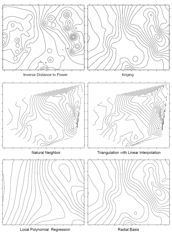
Different interpolation methods can result in different contour maps. Long range trend is common in environmental data sets and for some interpolation methods, the long range trend must be removed by detrending, described here, in order to obtain the best quality interpolation. Anisotropy occurs when the spatial correlation is different along different coordinate axes in the space and can also affect interpolation. Some interpolation methods take into account uncertainty in the measured data set. These methods, called inexact methods, may yield a contour map where a contour line may pass through a sampling point where the measured value is a little different from the value of that variable on the contour line.

▼Read more

Spatial or temporal interpolation methods predict values for a variable of interest at unsampled locations or time periods based on available data. Mathematical equations perform this interpolation and produce a continuous grid or time series of interpolated values. The underlying assumption common to all interpolation methods is that the measured values are spatially or temporally related; that is, values that are closer to one another in space or time will be more similar than values that are further away from one another (Webster and Oliver 2001). If this were not true, there would be no rational basis for interpolating between sampling locations.

The various interpolation methods available differ in the number of samples used in the model and how those results are weighted, and each method may produce a different result. In general, the result of interpolation is either a raster surface in which the interpolated values are assigned to grid cells, or an isocontour surface on which estimated values are connected to create non-intersecting lines. Spatial or temporal interpolation methods ideally produce predictions with the following characteristics (Krivoruchko 2011):

  • Predictions are based on measurements from nearby locations or time periods.
  • Predictions have associated measurements of uncertainty, and a model is chosen to minimize this uncertainty to the extent practicable.
  • Predictions can be converted to a probability of exceeding prescribed threshold values.
  • Predictions create smooth grids and contour maps without discontinuities.

Simple methods do not produce predictions with associated measurements of uncertainty. More complex and advanced methods are therefore inherently more powerful. In some cases, however, the simple methods may produce results that are similar to more complex methods. In addition, interpolation efficiency may be a more important project goal than rigorous uncertainty analysis. Often it is better to try multiple different interpolation methods and compare results to see which one is best suited to the current project needs.

For example, Figure 15 shows elevation contours of a clay aquitard using different interpolation methods available in Surfer (Kresic and Mikszewski 2012); see Methods for more information.

gro_fig_3_9

Figure 15. Contours of the elevation values for the top of a clay aquitard created by various contouring methods available in Surfer (Golden Software 2002).
Source: Kresic and Mikszewski 2012.

While the results of some methods may immediately appear unrealistic (for example, the bull’s-eyes produced by inverse distance to a power), it may be challenging to select the best method based solely on visual analysis. For example, the radial basis (spline) surface is similar to that produced by kriging. More rigorous comparison of the accuracy of different interpolation methods is typically performed through cross-validation and validation.

The extent to which interpolation methods use the spatial or temporal correlation of the data to account for uncertainty is only one aspect of the interpolation process. Additional characteristics of the overall interpolation process discussed in this section include:

  • long-range trend, anisotropy, and search neighborhood
  • exact versus inexact interpolation
  • interpolation boundary conditions
  • interpolation gridding

Long-Range Trend, Anisotropy, and Search Neighborhood

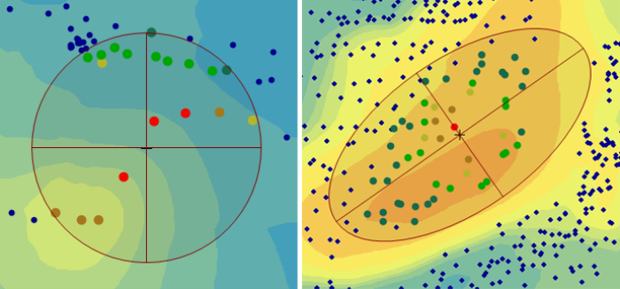
Environmental data commonly exhibit a long-range trend, which is typically expressed as a smooth, predictable change in values operating at a regional scale (Webster and Oliver 2001). Long-range trend is systematic and deterministic and is inherently variable, which affects kriging assumptions. Long-range trend should not be confused with geometric anisotropy, which is the directional dependence of spatial correlation. The search neighborhood defines the area over which data points are considered when interpolating a value at a new location.

Long-range trend▼Read more

Long-range trend is routinely observed in regional potentiometric surface data (Kitanidis 1997). This trend is observed because water level elevations are predominantly determined by hydraulic boundaries (such as high-elevation recharge zones) and low-elevation discharge zones (such as rivers). Contaminant concentrations in groundwater often exhibit long-range trend because plume orientation is largely determined by the potentiometric surface. The systematic increase in temperature moving from north to south (in the northern hemisphere) is another example of long-range trend (Krivoruchko 2011).

Long-range trend often creates the appearance of an infinite, unbounded range of spatial correlation, where the values appear to rise with no limits on a semivariogram plot (see Figures 10 and 16). Without reaching a limit (or “sill”) on the semivariogram, the range is indeterminant and the size of the neighborhood over which samples are related is unknown.

gro_fig_3_10

Figure 16. Semivariogram of water level elevations in ArcGIS Geostatistical Analyst.
Source: Kresic and Mikszewski 2012.

Figure 16 shows an infinite range of correlation, indicating the presence of trend and nonstationarity. The water levels in groundwater (red dots) exhibit a long-range trend because plume orientation is largely determined by the potentiometric surface. Long-range trend often creates the appearance of an infinite unbounded range of spatial correlation on a semivariogram plot, that is, continual climbing on the y-axis.

In some situations, interpolation of data with long-range trend using a simple geospatial method may satisfy project objectives. To apply kriging, removing long-range trend (detrending) may be necessary to approach stationarity and improve interpolation results (see advanced method assumptions). There should be conceptual justification for trend removal in geostatistics, however, because unnecessary detrending of data can yield worse results (Kitanidis 1997).

Polynomial regression is a common interpolation method that can also be used to detrend data sets prior to kriging the detrended residuals. This method fits polynomial equations to the data to generate a smooth (inexact) interpolated surface. Global polynomial interpolation is also known as trend surface interpolation because it fits one polynomial to the entire data set. Local polynomial interpolation divides the data set into moving windows around prediction locations, each of which has a unique polynomial equation (Krivoruchko 2011).

The differences between global and local polynomial interpolation output are illustrated in Figure 17. In the left map, a groundwater contaminant plume is interpolated using a second-order global polynomial equation. Using one equation to fit the entire data set results in an overly averaged surface that does not reflect the plume shape. In the right map (with the red circle), the same data set is interpolated using local polynomial interpolation. The surface better resembles a traditional plume shape.

gro_fig_3_11

Figure 17. Differences between global and local polynomial interpolation output.
Source: Kresic and Mikszewski 2012.

While the global interpolation model captures the long-range trend of concentrations rapidly declining away from the contaminant source area, it does not account for more local variation in the plume. In general, the surface produced by a global interpolation is not usable on its own for most applications in site remediation; see More Complex Geospatial Methods.

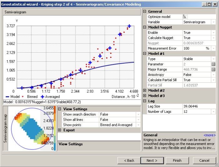
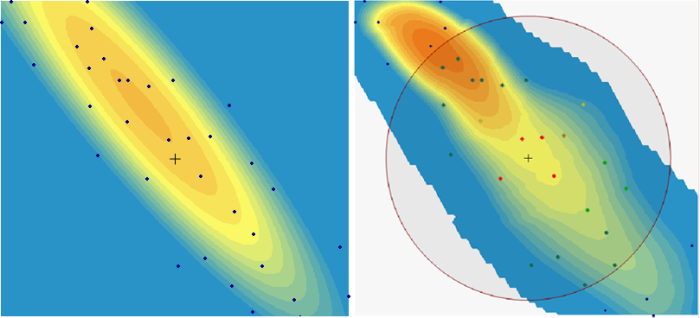
Geometric Anisotropy ▼Read more

is the directional dependence of spatial correlation. Stratified geologic formations provide the most common examples of anisotropy in environmental data. For example, interbedded layers of alluvial sediment deposits have horizontal orientations, meaning that physical properties such as hydraulic conductivity and storativity are more similar moving in the horizontal direction than in the vertical direction (Kitanidis 1997). Spatial interpolation models account for anisotropy by using an elliptical search neighborhood. The search neighborhood defines the area over which data points are considered when interpolating a value at a new location. A small search neighborhood emphasizes nearby measurements, and measurements outside the search neighborhood are excluded from the interpolation algorithm at that location. A circular search neighborhood emphasizes data points the same distance in all directions (Golden Software 2002).

An elliptical search neighborhood reflecting geometric anisotropy has different axis lengths (the ratio of which corresponds to the anisotropy ratio), and an orientation angle. The Surfer software manual (Golden Software 2002) states that “an anisotropy ratio less than two is mild, and an anisotropy ratio greater than four is severe.” However, for the previous example of variation in hydraulic conductivity in stratified formations, it is common to have anisotropic ratios greater than 10:1 when comparing horizontal hydraulic conductivity to vertical hydraulic conductivity. Even though mechanistic interpolation methods do not model spatial correlation, various computer programs such as Surfer and ArcGIS Geostatistical Analyst allow simulation of anisotropy using mechanistic methods such as inverse distance to a power. This simulation is performed by warping the coordinate system so that the distance in one direction changes faster than the distance in another in an elliptical manner (Krivoruchko 2011). The presence of anisotropy can also be assessed through analysis of the semivariogram, where the range and sill depend on search direction (see Spatial Correlation Models for Advanced Methods).

Search Neighborhood ▼Read more


defines the area over which data points are considered when interpolating a value at a new location. Figure 18 presents two different search neighborhoods to illustrate the concepts described above, one without anisotropy (left) and one incorporating an anisotropy ratio of 2 and an angle of 140 degrees (right). On the left, a circular search neighborhood is divided into four sectors. Hotter colors are given greater weight in the interpolation at the center of the circle, with small blue dots being excluded. On the right, elliptical search neighborhood incorporating anisotropy is shown. In this case a maximum number of data points to include within each sector is specified, resulting in the exclusion of small blue data points within the neighborhood but at its outer margin.

gro_fig_3_12

Figure 18. Two different search neighborhoods, one without anisotropy (left) and one incorporating an anisotropy ratio of 2 and an angle of 140 degrees (right).

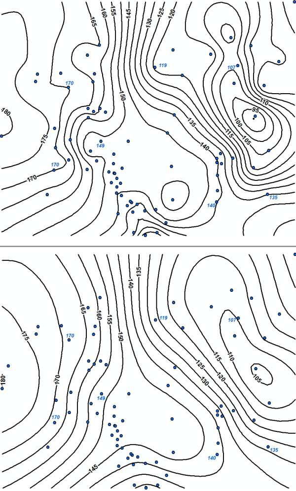
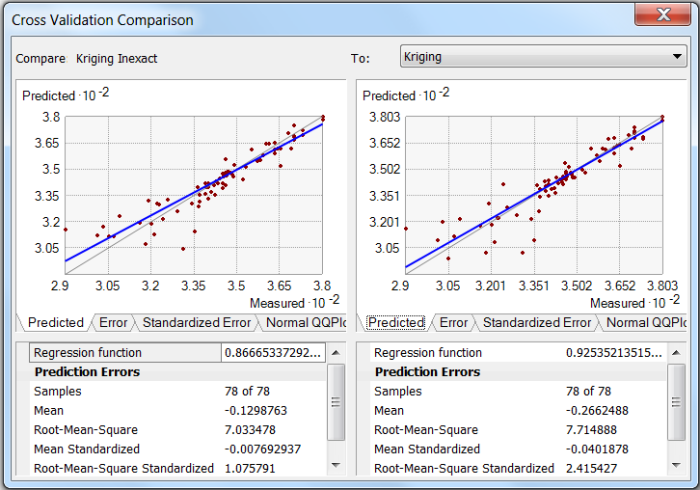
Exact versus Inexact Interpolation

Interpolation methods can either be exact or inexact interpolators. An exact interpolator produces values exactly equal to observed values at all measurement locations. In other words, an interpolated contour line with a value of 10 would exactly pass through all measurement points with value of 10. An inexact interpolator accounts for uncertainty in the data by allowing the model to predict values at sampling locations that are different from the exact measurements. In this case, a contour line with a value of 9 may pass through a measurement point with a value of 10. Inexact interpolators are often referred to as smoothing interpolators because they produce smoother surfaces with fewer discontinuities that better reflect the spatial correlation of the broader data set (Golden Software 2002). Conversely, exact interpolators are forced to honor each individual data point regardless of uncertainty or measurement error, often resulting in jagged contour lines or surfaces with bull’s-eyes.

▼Read more

The differences between exact and inexact interpolation are illustrated on Figure 19 (top and bottom), which presents two different kriging models for the clay aquitard data set in Figure 15. The top map shows exact kriging interpolation with a zero nugget (see further discussion of kriging and the nugget effect). Contours bend to exactly pass through corresponding measurement values. For example, see the labeled 135, 140, and 170 measurement values. The bottom map shows inexact kriging interpolation with a nugget that is significantly smoother. Note that the labeled 170 values are between the 165 and 170 contour lines, and the labeled 149 value is between the 150 and 155 contour lines.

gro_fig_3_13

Figure 19. Differences between exact and inexact interpolation.

Using exact interpolation models implies that the data have no measurement or locational error, which is unlikely on remediation projects. For these projects, laboratory analytical data have uncertainty observed through laboratory and field quality control samples such as field duplicates, laboratory duplicates, and surrogate recovery analysis. Furthermore, heterogeneity in subsurface geology can cause local variation in hydraulic head or contaminant concentrations. If measurements such as contaminant concentrations are accepted as imprecise, then there is no technical reason to use exact interpolation (Krivoruchko 2011). Exact kriging also causes the prediction and prediction standard error surfaces to be discontinuous, with predictions jumping to measured values and prediction standard error dropping to zero at measurement locations (Kitanidis 1997). This result creates a conceptual problem, and for most applications in site characterization and remediation it is beneficial to quantify uncertainty rather than ignore it. See the discussion of the use of advanced geospatial methods for this purpose.

When using inexact kriging with a nugget effect, the interpolation better evaluates the data set as a whole rather than over-emphasizing each individual measurement subject to this error. As a result, the overall accuracy of the inexact model as measured through cross-validation and prediction standard error is often better than the exact model.

Figure 20 presents a cross-validation comparison of the two surfaces presented in Figure 3-13 and demonstrates that the inexact model has less overall interpolation error.

gro_fig_3_14

Figure 20. Cross-validation results of the two kriging models using ArcGIS Geostatistical Analyst.

The inexact model (left) has a lower mean residual error, a lower root-mean-square error, and a root-mean-square standardized error closer to one (reflecting appropriate estimation of the variability of the data set). See additional discussion of cross-validation and interpretation of statistical metrics.

Despite the widespread acceptance of uncertainty in environmental data, inexact interpolations are frequently rejected by reviewers as being incorrect because contours do not exactly match data values. In spite of this practice, inexact interpolation models should still be considered because they can lead to more accurate quantification of metrics such as plume mass and well redundancy.

Most simple methods such as IDW and natural neighbor are exact interpolators that also will not interpolate beyond the range of data values. Polynomial regression interpolation is generally an inexact (smoothing) interpolator, while kriging can be exact or inexact depending on whether a nugget effect is included.


Interpolation Boundary Conditions (Breaklines, Barriers)

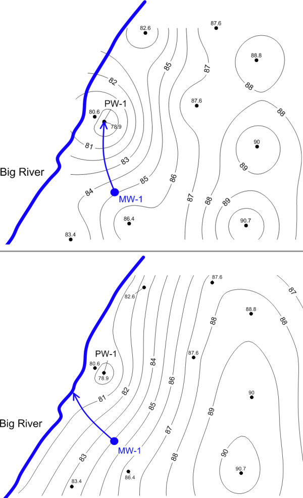
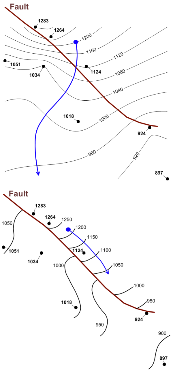
Spatial data at remediation sites are subject to boundary conditions that influence data orientation and correlation. The most common example is the influence of recharge and discharge boundaries on the groundwater potentiometric surface, which often results in long-range trend. Recharge boundaries may include injection wells, recharge basins, or losing streams, while discharge boundaries may include pumping wells, trenches and gaining streams. Another common boundary condition is a groundwater barrier, or no flow boundary. This barrier may include a bedrock contact, fault, or an engineered barrier such as a slurry wall or sheet pile. Boundary conditions can also produce other problems with the data set. These problems include edge effects, in which patterns of interaction or interdependency across the borders of the bounded region are ignored or distorted, and shape effects, in which the shape imposed on the bounded area affects the perceived interactions between phenomena (ESRI 2015a).

▼Read more


Beyond accounting for trend in a spatial interpolation model, boundary conditions themselves should be included in the interpolation, where appropriate, to more accurately reflect the physical processes influencing the data correlation. Head or concentration boundaries, such as streams and wetlands, can be included in an interpolation using a breakline, which is a defined line with X, Y, and Z values at each vertex. Barriers to flow or data correlation can be modeled as linear features across which the interpolation model does not exchange information. Surfer terms this line a fault, and data on one side of the fault are not directly used in the interpolation of data on the other side of the fault (Golden Software 2002). Interpolation with barriers can also be performed in ArcGIS, or manually in any software by interpolating data on different sides of the barrier separately and then joining the two surfaces together.

A common mistake when creating potentiometric maps of unconfined aquifers is to let a computer program ignore the presence of surface water features, which typically leads to erroneous results (Kresic and Mikszewski 2012). Figure 3-15 (top) presents an interpolated potentiometric surface map to evaluate the capture zone of a pump and treat well. The surface was created using inverse distance to a power interpolation without any representation of the Big River. A remedy optimization question for this application is whether pumping at extraction well PW-1 captures groundwater contamination at monitoring well MW-1. Based on the streamlines produced by this interpolation, it would be concluded that PW-1 does successfully capture this contamination.

Figure 21 (bottom) presents a kriging interpolation of the same data set with an X, Y, Z breakline file used to represent the elevations of the Big River. This surface shows groundwater at MW-1 to bypass PW-1 and discharge to the Big River. Based on this more defensible interpolation, the remedy may not be performing as designed and may require optimization and improvement.

gro_fig_3_15

Figure 21. Top: Inverse distance to a power interpolation of a synthetic data set created with a groundwater flow model. Bottom: Kriging interpolation of the same data set using a breakline to represent the Big River.

Note that the interpolation also shows the bull’s-eyes commonly associated with inverse distance to a power interpolation around other monitoring wells that are not pumping or injecting water. In the bottom map, the kriging interpolation shows that groundwater contamination at MW-1 is not captured by PW-1, which is erroneously indicated by the inverse distance to a power interpolation.

This example problem is a common situation at groundwater remediation projects where pump-and-treat is being used to prevent contaminant discharge to surface water. Geospatial analysis of these sites should incorporate surface water features to produce more accurate results.

A similar common error is contouring across faults and other barriers without considering the effect of the fault or barrier on the groundwater potentiometric surface, as shown in Figure 22 (top and bottom).

gro_fig_3_16

Figure 22. Top: Kriging interpolation of groundwater elevation data without considering the barrier effect of a fault separating two basins. Bottom: The georeferenced interpolated surface, correctly showing the influence of the fault as a groundwater barrier.
Source: Data from Woolfenden and Koczot 2001.

In the top map, the blue particle flow path is erroneously shown to flow across the fault. Note in the bottom map that in some places there is an interpreted head drop across the fault in excess of 100 feet.

The examples shown in this section highlight the importance of applying geospatial methods in a manner that is consistent with the CSM, which explains the underlying physical, chemical, and biological processes influencing the data.

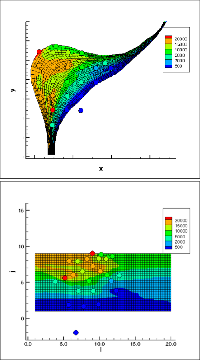
Interpolation Gridding

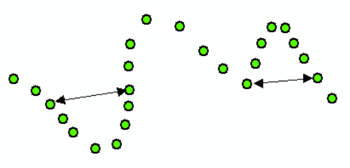
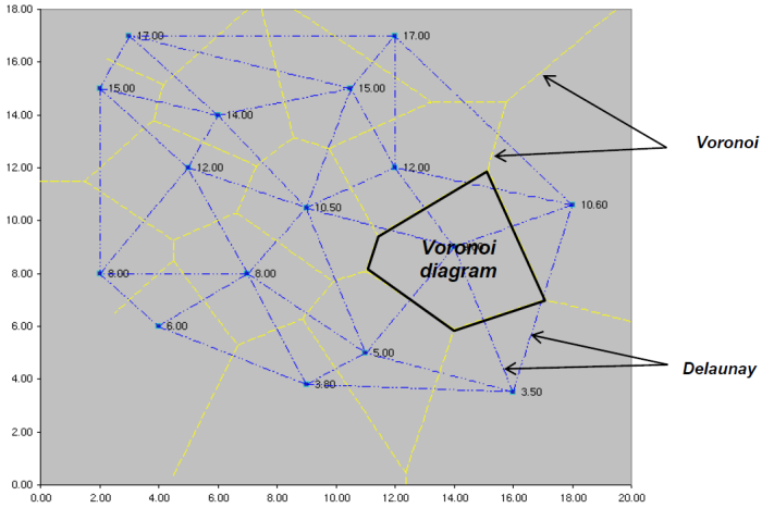
Regardless of the method used, the process of spatial interpolation with a computer program involves converting discrete point data (for example, monitoring well water level elevations or contaminant concentrations) to a continuous grid of predictions with at least one value associated with each grid cell. For example, a set of measured contaminant concentrations at specific well locations would be converted to a set of predicted contaminant concentrations at points across the grid. Such data on grids are termed raster data, and also may be referred to as surfaces. Grids produced by interpolation programs are typically square, but they may also be rectangular, curvilinear, or an unstructured finite element mesh. Delaunay triangulation is an example of a common unstructured grid used to generate a network of triangular shapes that are incrementally augmented through insertion of interpolated values into designated empty mesh cells. Several variations on the Delaunay algorithm exist and most are available in commercial modeling software through methods such as natural neighbor interpolation.

Delaunay triangles, Voronoi diagrams, Thiessen polygons

▼Read more

The Delaunay triangles are used to generate grids that divide space into cells called Voronoi diagrams or Thiessen Polygons. They are commonly used in software packages such as the Monitoring and Remediation Optimization System (MAROS) software, which uses Delaunay triangulation and Voronoi diagram spatial geometry for mesh generation. Delaunay triangulation creates a triangular mesh with all data points (typically spatial positions of monitoring wells) at its nodes. No point in the data set falls in the interior of the Delaunay triangles. The perpendicular bisectors of the Delaunay triangles form polygons termed Voronoi diagrams (also known as Thiessen polygons). A Voronoi diagram/Thiessen polygon contains the set of points on a plane closest to one specific data point in the network (GSI 2012). In other words, every location within a Voronoi diagram/Thiessen polygon is closer to the data point within that polygon than any other data point (ESRI 2013). A diagram illustrating Delaunay triangles and Voronoi diagrams/Thiessen polygons is provided in Figure 23; see additional details about the use of Thiessen polygons and Delaunay triangulation.

gro_fig_3_17

Figure 23. Illustration of Voronoi diagrams and Delaunay triangles for a data set in MAROS.
Source: GSI 2012.

Grid spacing

▼Read more

One of many advantages of the computer-based interpolation programs is that the grid file can be displayed in a variety of ways, including: contour lines at any interval, shaded contour maps at any interval, or as a three-dimensional surface. Grid files can also be transferred between various programs and used for quantitative purposes such as: calculation of volumes between surfaces, areas between contours, or surface gradients (slopes), or both. These mathematical grid operations have numerous applications in environmental project optimization, including:

  • calculating aquifer volume and contaminant mass in soil or groundwater
  • calculating changes in surface properties, such as changes in contaminant concentration between different time periods
  • creating layer surfaces for use in groundwater models (Kresic and Mikszewski 2012)

Interpolation methods require the specification of the resolution, or spacing, of the resulting grid file. The chosen grid spacing is a compromise between optimum density of information and efficiency—large grid cells provide less information but the model runs more quickly, while small grid cells increase the amount of information, but possibly at an unreasonable resource cost. Primary limiting factors are the number of known data points and the area over which the model is applied; generating many cells within a few known data points does not provide information that is any more accurate or representative than if fewer, larger cells are used.

Some software packages attempt to optimize cell size and present a default based on number of data points and breadth of the model. In general, the grid spacing should be appropriately scaled relative to the problem at hand. For example, a risk assessment of exposure to contaminated soils or sediments may require a certain grid spacing representing an exposure unit.

For most soil and groundwater applications, interpolation gridding is a relatively straightforward process in which computer programs generally recommend an acceptable default grid spacing. Conversely, spatial interpolation of sediment data often requires complex gridding to accommodate meanders or bends in a river. For example, a square or rectangular grid interpolation of the center-channel sediment data points depicted on Figure 24 may result in data points that are further away in terms of river mile, but closer in terms of distance in the X, Y plane, having a greater influence on the interpolation than those that are closer by river mile. Arrows designate points that are further by river mile but closer in the XY plane than other points.

gro_fig_3_18

Figure 24. Meanders in a river channel cause potential problems when interpolating to a regular grid.

To overcome this issue, a curvilinear grid may be used to convert coordinates to a rectangular i, j space corresponding to flow distance along the channel. After interpolating in the i, j space, the grid can be transformed back to rectangular X, Y space to display results in the desired projected coordinate system. This process is illustrated in Figure 25 (top and bottom).

gro_fig_3_19

Figure 25. Top: data plot of sediment and floodplain soil data in site X, Y coordinates depicting the curvilinear grid and the back-transformed interpolated surface. Bottom: transformed i, j coordinates along the curvilinear grid used to perform the interpolation.
Source: Grid design and transformation performed in Tecplot. Courtesy Jerry Eykholt, Amec Foster Wheeler.

Similar coordinate transformation of X, Y coordinates to i, j coordinates based on distance along the river bank or centerline can be performed in ArcGIS using linear referencing tools. Performing this type of grid-based coordinate transformation often results in improved variography and a much improved interpolation. More work may be needed, however, to refine settings, check the back-transformation, and provide uncertainty estimates. In addition, a higher sampling density may be required to achieve better spatial data coverage in the transformed i, j space.

image_pdfPrint this page/section


GRO

web document
glossaryGRO Glossary
referencesGRO References
acronymsGRO Acronyms
ITRC
Contact Us
About ITRC
Visit ITRC
social media iconsClick here to visit ITRC on FacebookClick here to visit ITRC on TwitterClick here to visit ITRC on LinkedInITRC on Social Media
about_itrc
Permission is granted to refer to or quote from this publication with the customary acknowledgment of the source (see suggested citation and disclaimer). This web site is owned by ITRC • 1250 H Street, NW • Suite 850 • Washington, DC 20005 • (202) 266-4933 • Email: [email protected] • Terms of Service, Privacy Policy, and Usage Policy ITRC is sponsored by the Environmental Council of the States.