Advanced Methods
This section presents an overview of advanced geospatial methods, which are used to estimate values at unsampled locations and model the spatial correlation of the data. These methods include varieties of kriging and conditional simulation. Kriging is a spatial interpolation method that allows estimation of values at unsampled locations and provides an estimate of the uncertainty in the interpolated values. Selection of a particular kriging method depends on the characteristics of the data set, such as trends present in the data or the degree of spatial correlation, which can be determined using variograms and other spatial correlation models. Information about using spatial correlation models, different kriging methods, and conditional simulation is also presented in this section.
Spatial Correlation Models for Advanced Methods
Kriging and simulation methods require a model of spatial correlation. Spatial autocorrelation can be modeled using the variogram or covariance function. Typically, the empirical variogram is plotted based on the data, and a variogram model is fit to the empirical variogram. These activities may be referred to as variography. In general, variography encompasses directional spatial autocorrelation, bivariate autocorrelation, and multivariate spatial autocorrelation.
Most advanced geospatial methods rely on a search neighborhood to generate spatial predictions. The search neighborhood is selected based on the underlying spatial autocorrelation in the sampled population, and is simply the radius within which known values are used to predict unknown variables. Recognizing that correlation decreases with distance, the optimal search neighborhood is one which includes known values with a large influence and excludes the rest.
Construction of the Empirical Variogram
As part of EDA, the empirical variogram is constructed by plotting one-half the squared difference in values (semivariance) for each pair of sampling points as a function of distance separating the points (variogram cloud; see Figure 78). The variogram expresses the variability of the data set as a function of space: if data are spatially correlated, then on average, close sample points are more alike and have a smaller semivariance than samples farther apart.
The choice of the variogram parameters (for example, lag, direction) is a fundamental step for using advanced geospatial methods and should be done so as to be as representative as possible of the spatial characteristics of the data set. For example, if anisotropy is observed, which is common in environmental data, then an anisotropic variogram must be built that takes into account different spatial directions. Experimental variogram parameters are intrinsically linked to each particular data set; nevertheless, some recommendations can be made in order to create a suitable experimental curve.
Lag
When sampling is performed by following a regular grid, the regular distance between samples is taken as the value of the variogram lag. Distance between samples, however, is often irregular and the lag of the variogram then may be chosen by taking into account the different distances between the pairs of sampling locations. In this case, the value of the lag may be calculated by taking the average of distances between the sampling locations. As the distance between samples becomes larger, the reliability of the estimates of semivariance goes down. Consequently, a rough rule of thumb is that the maximum lag distance should not exceed half of the maximum distance between samples (see Figure 76).
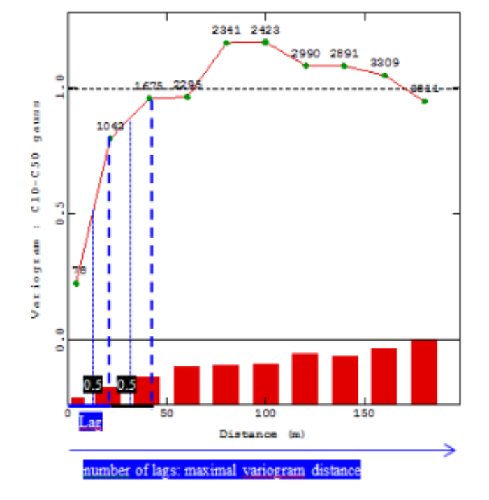
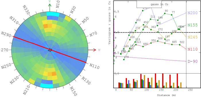
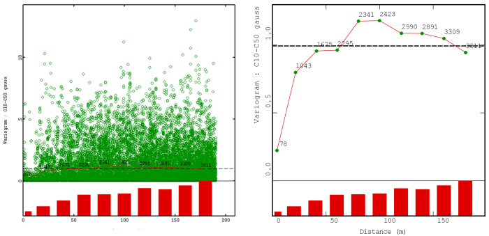 Figure 78.
 Fitting the Empirical Variogram
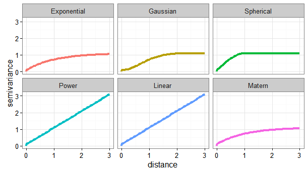
The fitting model chosen is used to calculate the data values (for example, contaminant concentrations) at each modeled point. Therefore, a model must be created that is as representative as possible of the data and, by extension, of the experimental variogram previously constructed. The data set characteristics can guide the choice of the model to be used.
Kriging
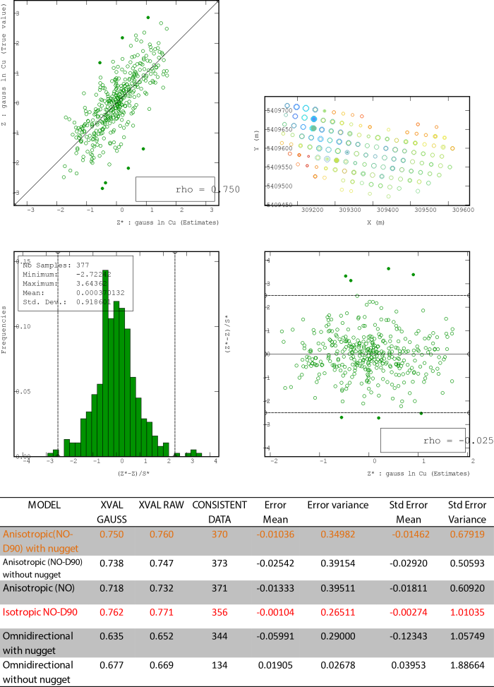
Kriging often relies on an optimal search neighborhood to generate spatial predictions. The optimal search neighborhood is determined by the underlying spatial autocorrelation in the sampled population. In general, kriging uses sampled values, within a pre-defined search neighborhood (defining the maximum and minimum number of “neighbors” to use), to estimate values at unsampled locations with a measured degree of confidence (called the kriging variance). The search neighborhood is optimized through evaluation of the semivariogram (univariate case) or cross-variogram (multivariate case). Because kriging uses an optimized search neighborhood for generating spatial estimates (the variogram is used to identify the distance over which properties are correlated), it is highly sensitive to the sample coverage, sample support, sample interval, and extent, which should be considered during the sampling design phases.
Data Transformations
Point and Block Kriging
Simple Kriging
Simple kriging assumes that the mean of the data is constant and known, which is a restrictive assumption. Consequently, ordinary kriging is preferred because it assumes that the mean is unknown and must be estimated from the data. Simple kriging is not recommended to be used by itself, but is regularly applied in conditional simulation.
Typical Applications
Using this Method
Assumptions
Strengths and Weaknesses
Understanding the results
Ordinary Kriging
Ordinary kriging assumes that the overall mean is constant, though unknown, and the variance is finite (the variogram has a sill value). The goal is to produce a set of estimates for which the variance of the errors is minimized. To accomplish this goal, ordinary kriging weights each sample based on its relative distance from the location of the data point to be predicted.
Typical Applications
Using This Method
Assumptions
Strengths and Weaknesses
Understanding the results
Further Information
Universal Kriging and Kriging with External Trend
Alternatives to ordinary kriging are universal kriging and kriging with external trend. Kriging with external trend is also known as kriging with external drift. These methods do not assume that the mean is constant, or even known, and assume that the trend that predicts the value of Z(s) can be modeled using a simple linear regression. If the linear regression for the trend uses only the spatial coordinates (for example, easting and northing) as explanatory variables, the method is called universal kriging. The form of regression commonly used with universal kriging is linear or quadratic, but any form can be used. Both the regression coefficients and kriging weights are estimated simultaneously by universal kriging.
If the regression uses other quantities as explanatory variables, the method is called kriging with an external trend. For example, the drawdown around a pumping well can be predicted using the Theim equation, which is a function of the distance from the pumping well. The trend in groundwater levels near the well can be included in the kriging method using a regression form of the Theim equation, with distance to the well as the explanatory variable. Kriging with an external trend fits the measured water levels at monitoring wells by adjusting both the regression coefficients and the kriging weights.
Typical Applications
Using this Method
Assumptions
Strengths and Weaknesses
Understanding the Results
Further Information
Indicator Kriging
Indicator kriging method is a nonparametric variant of ordinary kriging using data indicator variables that are defined using binary values (0 or 1) based on whether the data exceed a specified threshold (such as the remediation goal). The value assigned to the sample points exceeding the specified threshold is 1. The assigned value is 0 for the sample points below this threshold.
Typical Applications
Using this Method
Assumptions
Strengths and Weaknesses
Understanding the results
Other Kriging Methods
Probability Kriging.▼Read more
Disjunctive Kriging▼Read more
Regression Kriging.▼Read more
Factorial Kriging Analysis (FKA)▼Read more
Co-kriging
In general, co-kriging is used only when the primary variable is under-sampled and the secondary data are spatially correlated with the primary variable (Goovaerts 1997). Direct measurements, such as those obtained from soil cores and geologic borings, are also referred to as primary sampling and are often limited in spatial coverage because of their cost, accessibility requirements, manpower, or invasiveness. Sparse direct measurements can prove inadequate for capturing the underlying spatial or temporal autocorrelation of a property or process of interest. When primary sampling is limited, it can be advantageous to incorporate secondary sampling technologies as supplementary site characterization tools. An example application of co-kriging is included.
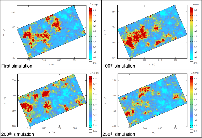
Conditional Simulation
Conditional simulation is the most robust way to create exceedance probability maps. A major limitation to kriging techniques is that the methods minimize the variance to generate the spatial estimates. This result inherently underestimates the variability of the system being characterized and biases the probability outcomes. Conditional simulation is a nonlinear method designed to produce fields showing the same spatial structure (variogram) and the same histogram as the original data. The simulations must ensure that each field is consistent with the observed values on the sample points if the nugget value is zero. Thus, if a value is simulated at a point coinciding with an observation, the simulated value must be equal to the observed value.
Sequential Gaussian simulation is the most commonly used method to develop conditional simulations and is included in several software packages.
Sequential Gaussian Simulation
This method generates each x value one-by-one by using kriging. Values are based on the kriging mean and variance obtained at the location xi from the data. The term Gaussian is derived from the use of normal (Gaussian) conditional distributions, functions, and parameters.
The basic approach of sequential Gaussian simulation is to generate a random path for each point to simulate. This method generates a conditional distribution which is also a Gaussian (normal) distribution, whose expectations and variances can be deduced from simple kriging. The sequential Gaussian simulation method transforms the bivariate distribution into a univariate distribution. The size of the kriging increases with each additional simulated point. Kriging can be limited to a moving neighborhood; however, errors (artifacts) may occur if the neighborhood is too small.
Typical Applications
Using this Method
Assumptions
Strengths and Weaknesses
Understanding the Results

Further Information

