Extent of Radiological Contamination in Soil at Four Sites near the Fukushima Daiichi Power Plant, Japan (ArcGIS)
Contact: Ted Parks, AMEC Foster Wheeler, [email protected], Alex Mikszewski, AMEC Foster Wheeler, [email protected]
Problem Statement
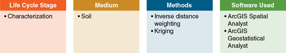
This case study illustrates the use of ArcGIS interpolation and spatial statistics tools to delineate the extent of contamination and required remediation at four sites in response to the 2011 radiological release at the Fukushima Daiichi nuclear power plant. This project was completed as part of a demonstration of Orion ScanPlot technology (ScanPlot) (AMEC Foster Wheeler 2015). ScanPlot technology is a mobile data-collection system for surface and shallow-depth radiological examination and characterization of open land. ArcGIS tools were used to process and analyze the ScanPlot data to produce maps of detected radioactivity, including concentrations of individual radioactive isotopes, to inform site remediation activities.
Site Background
Assessment and remediation activities were completed at four separate areas within a 20 km radius around the Fukushima Daiichi nuclear power plant. These areas were located in schoolyards, roads, and agricultural fields. Due to variable terrain of the areas, ScanPlot was deployed in three different configurations: a “buggy”, back-pack unit, and truck-mounted unit (see Figure 103).
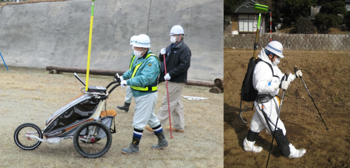 Figure 103. ScanPlotSM “buggy” (left) and back-pack deployment (right).
Project Objectives
The primary objective was to delineate the spatial extent of soil contamination and optimize remedial decision making at the four study areas. To accomplish this objective, data obtained from ScanPlot was mapped and spatially analyzed during the field investigation using ESRI’s ArcGIS platform. Geospatial interpolation of the data was used to compute zonal statistics and identify areas above risk-based criteria. A secondary objective of the geospatial analysis was to evaluate the conceptual model for radiological contaminant transport and deposition. Following remediation, interpolation and data plotting verified that cleanup levels were achieved.
Data Set
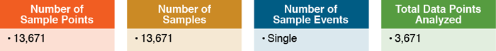
At each study area, radiological contaminant levels and corresponding GPS locations were measured at high density on an approximate 1 m grid, resulting in thousands of data points measuring cesium-137 exposure levels in microsieverts per hour (uSv/hr). Over 13,000 data points were collected. Data from ScanPlot was imported into ArcGIS and plotted using the coordinates collected by the GPS component of the system. IDW interpolation was used in the Spatial Analyst extension to rapidly and accurately contour and visualize the data.
Methods
Data plots were generated as the data were collected during the field assessments. The interpolated surfaces informed the ScanPlot locations and ultimately the remedial footprint delineation. IDW was a good interpolation method for this task because of the large volume, high-density, and even distribution of the data. IDW in Spatial Analyst can contour up to approximately 45 million data points.
The resulting maps provided visualizations of the distribution of radiological contaminants. The maps showed that the contamination existed across the sites with relative uniformity. This result was consistent with the expected fall-out delivery method of the contamination. Sites with more variable topography or pronounced drainage features exhibited signs of surface water transport of radioactive materials. Higher levels of contamination were found in ditches and low-lying spots, presumably washed there by runoff. Sites higher in elevation and more exposed to wind showed overall higher concentrations than those in low-lying areas that were partially shielded by topographic features.
Example contour maps of cesium-137 exposure levels in microsieverts per hour (uSv/hr) for two ScanPlot surveys are presented on Figure 104 (left and right).
To optimize remedial decision making, AMEC used the ArcGIS Zonal Statistics tool set to calculate the mean of the IDW interpolated data for a 10 m grid covering the sites. This approach was used to identify portions of the site to excavate where average levels exceeded risk-based criteria. In targeting just these areas, responders could have avoided removing soil over the entire site and still achieved acceptable exposure-point contamination levels. Maps created using the Zonal Statistics tool set in the Spatial Analyst Extension are presented in Figure 105 (left and right).
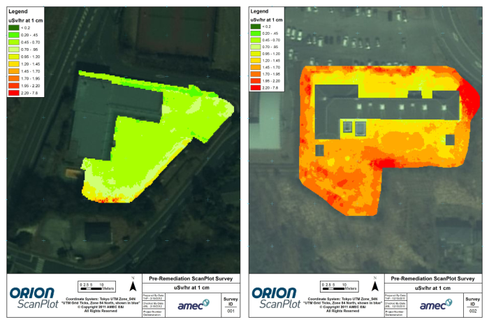 Figure 104. Maps of cesium-137 levels created using ESRI’s Spatial Analyst Extension.
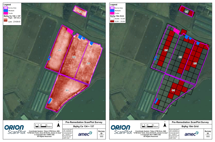 Figure 105. Left: Average combined cesium-134 and 137 levels created using the Zonal Statistics tool set. Right: Identification of 10-meter grid cells (red) with levels exceeding risk-based thresholds (red).
Due to the sensitivity of the receptors (farmland and schools), regulatory officials conservatively decided to excavate the entirety of the sites to a depth of 10 cm. Following remedial activities, the sites were scanned a second time. The results of the postremediation scan verified the effectiveness of the remedial activities in reducing levels to below risk-based criteria. Postremediation contour maps generating using IDW in Spatial Analyst are presented in Figure 106 (left and right).
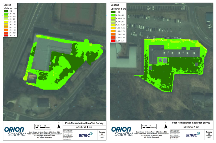 Figure 106. Maps of postremediation cesium-137 levels created using ESRI’s Spatial Analyst Extension.
More advanced analysis and interpolation of the radiological data can be completed using ESRI’s Geostatistical Analyst extension. This extension has a robust set of data exploration tools, including histogram, trend, and semivariogram analysis, to characterize the data set for stationarity, a required condition for kriging. Data are stationary if there is a constant mean and variance across the data domain, and data correlation depends only on separation distance and direction, rather than absolute location. An implicit assumption commonly accepted by statisticians is that kriging requires data to be normally distributed, or that it can be transformed to approximately follow a normal distribution. The data exploration utility in Geostatistical Analyst enables the user to understand how to transform data to improve kriging estimates and reduce interpolation error.
Figure 107 (left and right) illustrates the histogram utility in Geostatistical Analyst, while Figure 108 illustrates the trend analysis utility.
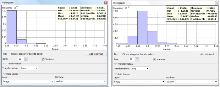 Figure 107. Left: histogram of raw cesium-137 data for one of the ScanPlot sites. Right: histogram of log-transformed data better resembles a normal distribution.
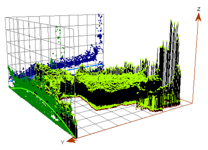 Figure 108. Trend visualization in Geostatistical Analyst with the Z-axis representing cesium-137 levels.
Strong trends are evident moving from high levels to low levels, implying large-scale, deterministic correlation of the data. This trend is likely related to runoff-mediated transport of contaminants.
The knowledge gained from performing data exploration can be applied when implementing kriging interpolation in Geostatistical Analyst. First, Geostatistical Analyst can log-transform the data prior to variography. Then, the second-order trend surface observed in Figure 107 can be removed from the data. This trend surface is presented on Figure 108. With these two steps, the data better approximate stationarity, with a constant variance (sill) evident on the semivariogram depicted in Figure 109.
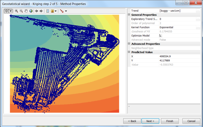 Figure 109. Detrending utility in Geostatistical Analyst.
Removing a second order polynomial equation from the data set places kriging emphasis on local variability rather than large-scale boundary effects. Data point locations are presented in blue. Kriging occurs on the residuals remaining from the detrending. In this case a “stable” semivariogram model is used, which is a hybrid between typical Gaussian and Exponential models. Note anisotropy can be incorporated into the model, but in this case is omitted.
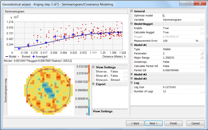 Figure 110. Semivariogram fitting utility in Geostatistical Analyst.
The resulting kriged surface is presented on Figure 111 (left), and is very similar to that previously produced using IDW interpolation (right). This similarity is expected given the high density of data collection. Geostatistical Analyst automatically back-transforms data to the final raster surface, so the user does not need to manually adjust for the prior log-transformation and detrending. The IDW surface appears smoother and performs more averaging in areas with higher measured levels.
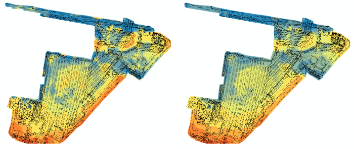 Figure 111. Left: interpolated Cesium-137 surface created using ordinary kriging with log-transformation and detrending. Right: interpolation surface created using IDW.
Geostatistical Analyst automatically performs cross-validation on spatial interpolation models and summarizes the results for the user. Cross-validation allows assessment of the accuracy of an interpolation model by computing and investigating the gridding errors, also referred to as residuals. The gridding errors are calculated by removing the first observation from the data set, and using the remaining data and the specified model to estimate a value at that location. The difference between the data value and the estimated value is the residual. This process is repeated for each individual data value and summary statistics (for example, mean error, root-mean-square error) are then calculated for the residual data set.
For kriging models, Geostatistical Analyst also provides the prediction standard error, or prediction standard deviation (same units as data), of each prediction location. This enables calculation of three additional metrics during cross-validation: mean standardized error (dimensionless), average standard error (analogous to root mean square error), and root-mean-square standardized error (measuring the assessment of prediction variability).
Beyond visual comparison, the performance of kriging versus that of IDW can be evaluated using cross-validation statistics. Geostatistical Analyst has a compare models utility that summarized cross-validation results for different models and plots them side-by-side. A screen-shot of this utility comparing the two interpolated surfaces presented in Figure 111 is presented in Figure 112.
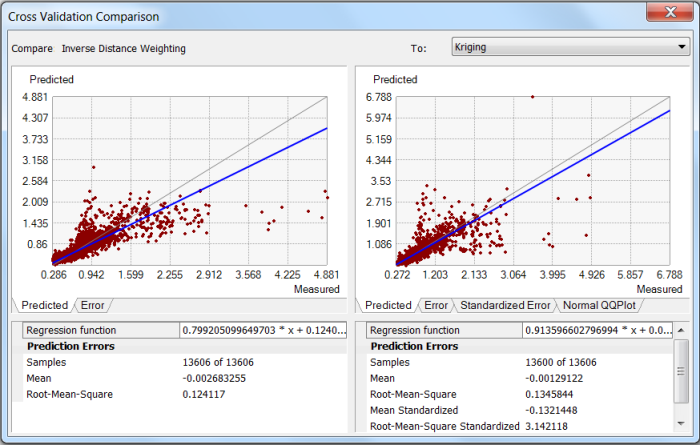 Figure 112. Cross-validation comparison of kriging versus IDW in Geostatistical Analyst.
Kriging has a lower mean residual error and a slightly reduced bias compared to IDW. However, IDW has a lower root-mean-square error, demonstrating its suitability for rapid interpolation of high density data. Note that standardized statistics are not available to deterministic models such as IDW that are not based on spatial correlation of the data. The root-mean-square standardized error for the kriging model would ideally be closer to one, indicating that the kriging model could be improved with additional analysis and revision.
Results
The Spatial Analyst extension to Esri’s ArcGIS was used to rapidly interpolate between thousands of data points collected during assessment of four sites impacted by the radiological release at the Fukushima Daiichi nuclear power plant. These interpolations were performed while field investigations were ongoing in order to inform additional data collection efforts. Zonal statistics were calculated on the interpolated surfaces in Spatial Analyst to develop risk-based remedial optimization scenarios. Advanced data analysis performed in Geostatistical Analyst confirmed the presence of trend and spatial correlation in the preremediation data set and validated the original IDW interpolations. Postremediation (soil excavation) scanning demonstrated the successful elimination of the areas of greatest concern identified using zonal statistics.

