Example 1
| Example 1: Sampling Redundancy Analysis in Visual Sample Plan (VSP) |
|---|
|
Application: Monitoring Program Optimization
Application Summary: The sampling redundancy module in VSP was used to identify redundant wells for a semiannual water level gauging program, and to identify a statistically defensible sampling frequency for metals analysis. Methods: Well redundancy analysis using global kriging weights and root mean square error (RMSE) analysis, temporal variogram analysis for temporal optimization. Data Requirements: VSP guidance recommends at least 30-50 data points for well redundancy analysis, and 20-30 observations for temporal variogram analysis. Reference: Matzke et al. 2014 |
|
Approach: The well redundancy analysis requires fitting a variogram using a normal score transform of the data to accommodate skewed data (see Figure 50). After the user kriges the data, VSP determines a global kriging weight for each well by adding the kriging weights for that data point for all locations in the kriging grid. The wells with higher global kriging weights have greater impacts on the interpolation. VSP then ranks the wells by their global kriging weight, the lowest ranked data location is removed from the data set, and the remaining data are kriged. This process is repeated until the maximum number of wells is removed from the data set. At each step, VSP calculates the root mean square error (RMSE) between the base interpolation with all wells, and the interpolation generated at that step. A graph of RMSE versus wells removed can then be used to determine a reasonable number to remove without significantly reducing the accuracy of the interpolation (see Figure 51). To support this decision, the user can visually compare maps of the base case (all wells) to those generated after eliminating any number of wells; see Figure 52 (Matzke et al. 2014). The sampling frequency analysis involves completing single well variography to evaluate the range of temporal correlation at each well. The fitted range parameter conceptually represents the minimum time interval between independent sampling events (see Figure 53). Note that VSP also has an iterative thinning module for temporal optimization that is described in the ITRC GSMC-1 guidance document.
Results: The well redundancy analysis indicates that approximately 30 wells may be removed from the gauging program without significantly affecting the accuracy of the interpolation. The range of temporal correlation of the data is greater than 365 days, supporting a reduction in sampling frequency from semiannual to annual. |
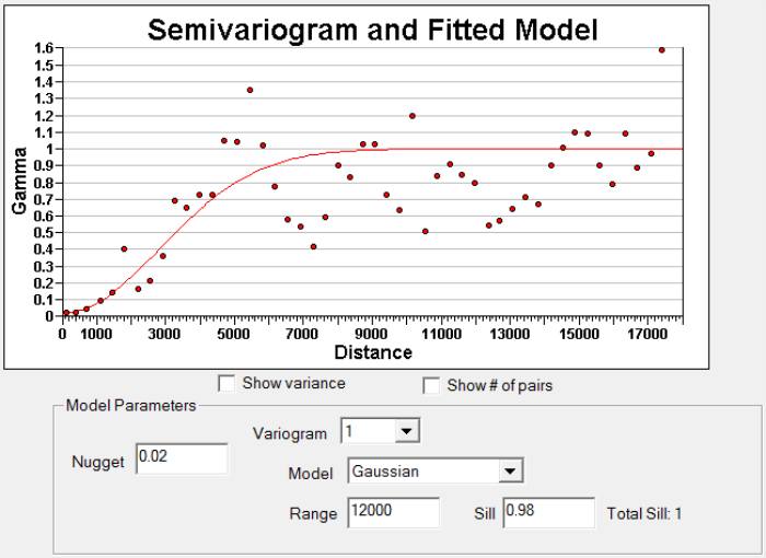
Figure 50. Example fitted model for the semivariogram of normal scores of the water level data.
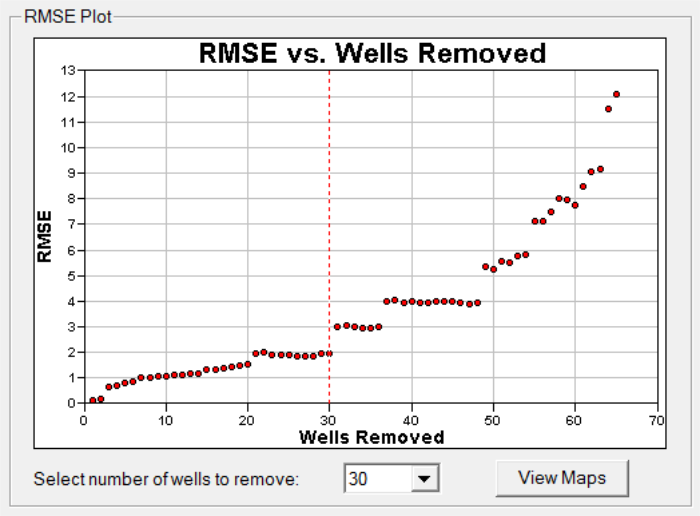
Figure 51. RMSE error plot versus wells removed. A companion table links well identifiers to RMSE results.
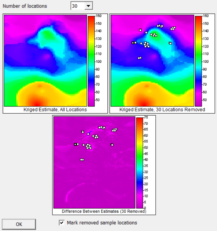
Figure 52. Comparison of interpolation maps using all locations and the trimmed data set.
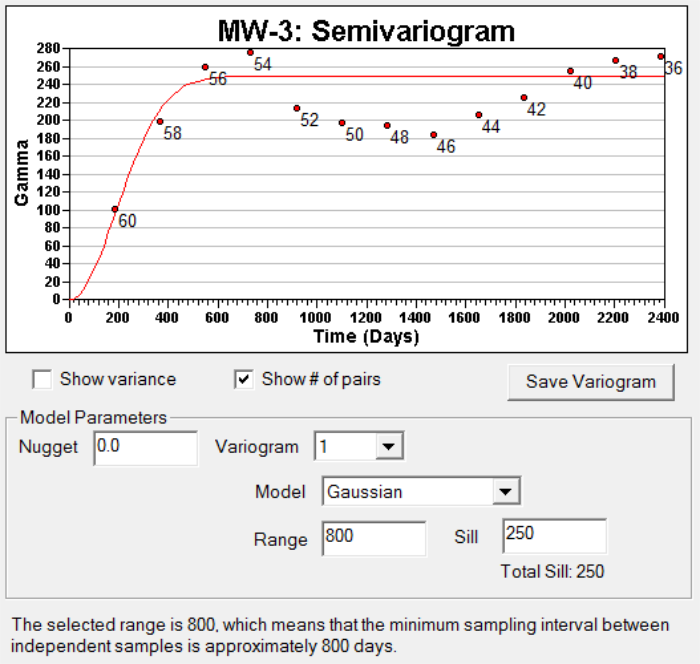
Figure 53. Variogram analysis for arsenic (As) at well MW-3, with estimated range of 800 days.

