• Skip to main content
itrc_logo

Geospatial Analysis for Optimization at Environmental Sites

Navigating this Website
Overview
Fact Sheets
Fact Sheets Overview
Fact Sheet 1: Do You Need Geospatial Analysis?
Fact Sheet 2: Are Conditions Suitable for Geospatial Analysis?
Fact Sheet 3: How is Geospatial Analysis Applied?
Fact Sheet 4: What Software is Available to Help?
PM's Tool Box
PM's Tool Box Overview
Review Checklist
Choosing Methods
Common Misapplications
Optimization Questions
Geospatial Analysis Support for Optimization Questions in the Project Life Cycle
Data Requirements
General Considerations
Methods for Optimization
Geospatial Methods for Optimization Questions in the Project Life Cycle Stages
Release Detection
Site Characterization
Remediation
Monitoring
Closure
Documenting Results
Fundamental Concepts
Fundamental Concepts for Geospatial Analysis
Basic Data Concepts for Geospatial Analysis
Interpolation Methods and Model Prediction
Uncertainty in Geospatial Analyses
Characteristics of Interpolation Methods
Work Flow
Work Flow for Conducting Geospatial Analysis
Geospatial Analysis Work Flow Overview
Perform Exploratory Data Analysis
Select Geospatial Method
Build Geospatial Model
Evaluate Geospatial Method Accuracy
Generate Geospatial Analysis Results
Using Results
Using Analysis Results for Optimization
Plume Intensity and Extent
Trend Maps
Estimating Quantities
Hot Spot Detection
Sample Spacing
Estimating Concentrations Based on Proxy Data
Background Estimation
Quantifying Uncertainty
Remedial Action Optimization
Monitoring Program Optimization
Examples
Examples Overview
Example 1
Example 2
Example 3
Example 4
Methods
Methods Overview
Simple Geospatial Methods
More Complex Geospatial Methods
Advanced Methods
Index of Methods
Software
Software Overview
Software Comparison Tables
Software Descriptions
Workshops and Short Courses
Case Studies
Case Studies Overview
Superfund Site Monitoring Optimization (MAROS)
PAH Contamination in Sediments—Uncertainty Analysis (Isatis)
Optimization of Long-Term Monitoring at Former Nebraska Ordnance Plant (GTS; Summit Envirosolutions)
Optimization of Lead-Contaminated Soil Remediation at a Former Lead Smelter (EVS/MVS)
Extent of Radiological Contamination in Soil at Four Sites near the Fukushima Daiichi Power Plant, Japan (ArcGIS)
Optimization of Groundwater Monitoring at a Research Facility in New Jersey (GWSDAT)
Optimization of Sediment Sampling at a Tidally Influenced Site (ArcGIS)
Stringfellow Superfund Site Monitoring Optimization (MAROS)
Lead Contamination in Soil (ArcGIS)
Stakeholder Perspectives
Additional Information
Project Life Cycle Stages
History of Remedial Process Optimization
Additional Resources
Acronyms
Glossary
Index of Methods
Acknowledgments
Team Contacts
Document Feedback


Geospatial Analysis for Optimization at Environmental Sites
HOME

More Complex Geospatial Methods

This section includes information on more complex geospatial methods such as parametric regression, splines and kernel smoothing, nonparametric regression and multiple regression. These methods offer some potential advantages over the simple methods because they allow predictions from the data and estimate the uncertainty of those predictions. The assumptions, strengths, and weaknesses of each method are described, as well as guidance on using the method results. An example at the end of this section illustrates how the results of these geospatial methods can be applied to address specific optimization questions.

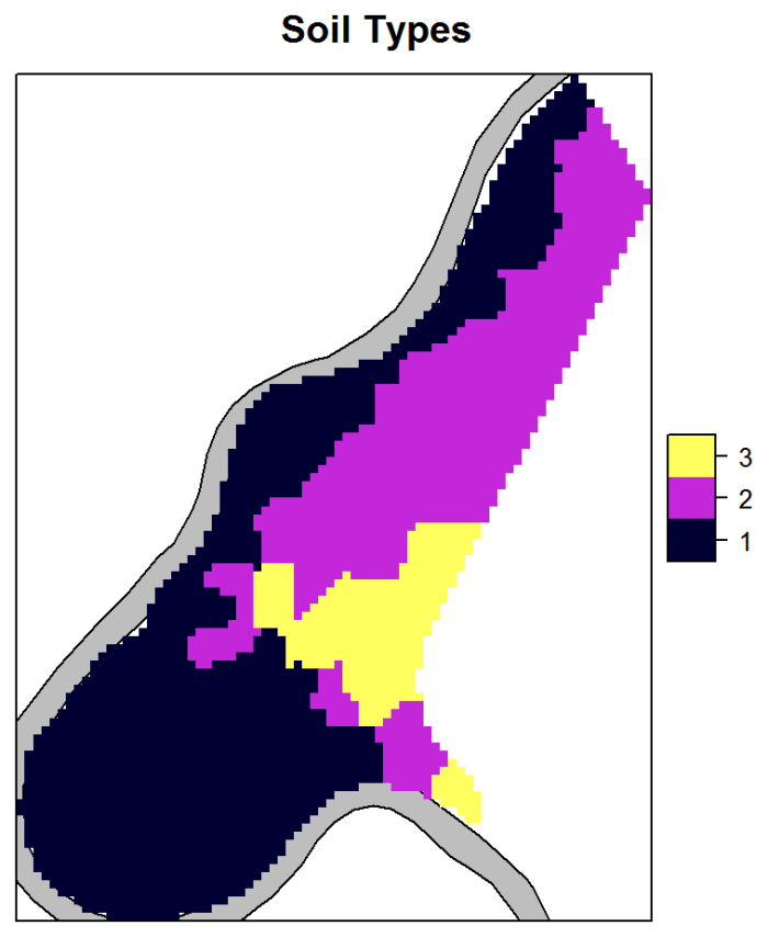
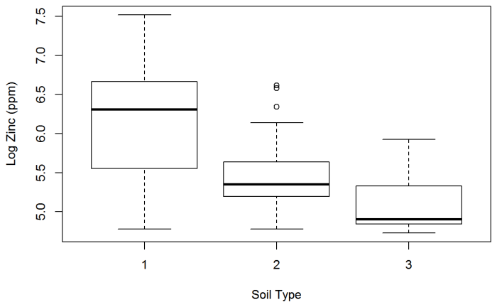
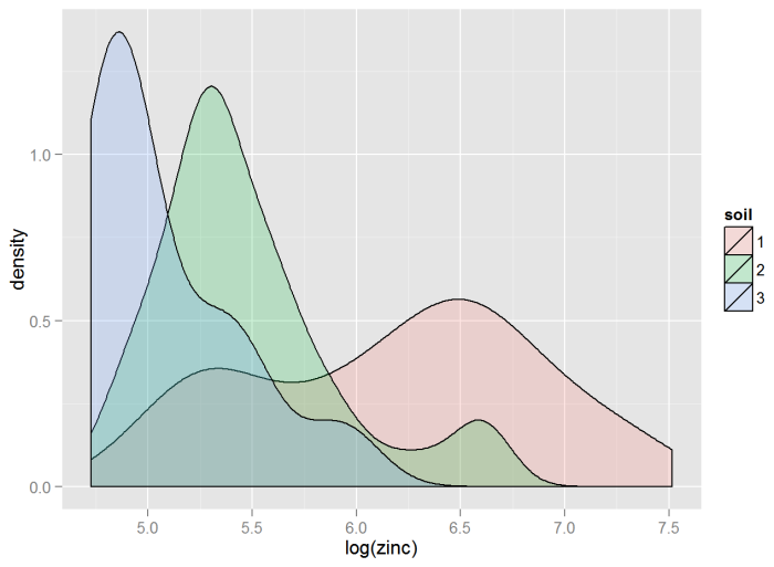
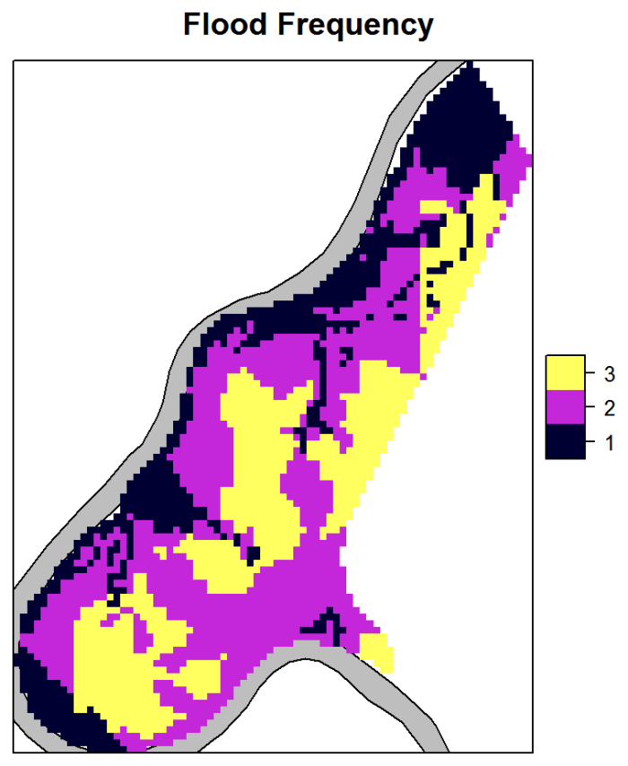
These methods can predict values for the variable of interest based on functions of the coordinates, but they work best when additional explanatory variables are available. Explanatory variables can include almost any type of information that is related to the quantity of interest, even data that are categorical (for example, soil type).

Methods based on splines and kernel smoothing are extremely flexible and can be used to accommodate physically important features in mapping such as break lines and barriers. Spline methods can produce maps that account for autocorrelation in a way that is equivalent to kriging (Wahba 1990). The main difference between splines and kriging is how the degree of smoothing is estimated and how uncertainty estimates are provided. Nonparametric regression uses spline and kernel smoothing methods within a regression framework.

Multiple regression allows the examination of the relationship between multiple variables associated with each point or unit of observation (concentration, soil type). Any variable can be a function of any other variable measured on the same sample. Multiple regression is a useful tool with which to examine relationship among the variables and to predict the value of one variable based on the known values of the other variables. The regression example illustrates various regression approaches.

Parametric Regression

Global parametric linear regression (which includes all the relevant data from the site) fits a simple polynomial function of the data coordinates and possibly other explanatory variables. This approach is often called “trend surface analysis” when fitting low-order polynomial functions of the coordinate variables. The surface generated by the polynomial changes gradually and captures the large-scale (global) pattern in the data. Trend surface analysis on its own may be too simple to create useful maps in most cases, but when it is combined with kriging it is a powerful method. The methods available for combination include universal kriging, kriging with an external trend, and regression-kriging.

There are many available modifications to the traditional linear regression method that extend its flexibility and usefulness. In particular, generalized linear models (GLMs) allow the modeling of non-normal distributions and accommodate a degree of non-linearity in the model structure. These methods are not described in this guidance. An introduction to these methods is provided by Dobson (2001), and the comprehensive reference is McCullagh and Nelder (1989).

Assumptions

▼Read more

Parametric regression analysis assumes the following:

  • The error is a random variable with a mean of zero, conditional on the explanatory variables.
  • The independent variables are measured with no error.
  • The predictors are linearly independent; it is not possible to express any predictor as a linear combination of the others.
  • The error terms are uncorrelated, that is, the variance–covariance matrix of the error terms is diagonal and each nonzero element is the variance of the error.
  • The variance of the error is constant across observations (homoscedasticity).

Strengths and Weaknesses

▼Read more

This method is a simple way to model large-scale trend and can include additional explanatory variables to improve predictions. This method cannot be used to model complex surfaces unless additional explanatory variables are included that explain most of the variation.

Understanding the Results

▼Read more

In the context of optimization, see how to use the results of the geospatial methods to address specific optimization questions.

Splines and Kernel Smoothing

Spline and kernel smoothing methods represent a wide class of smoothing interpolation methods. One method of interpolation is to fit a polynomial surface the measured data points, where a global polynomial encompasses the entire area of interest, but may not contain sufficient detail to capture small scale variations. Local polynomials can be used to capture small scale variation, but they may not apply universally. A piecewise polynomial fitting combines adjacent local polynomial models into a patchwork model; the models can be generated using different polynomial functions but their boundaries must line up for an even joining.

Aligning boundaries is accomplished through the use of splines, which describe how the joined model behaves at the boundary between the different polynomial functions. Splines allow a smooth transition and a flexible interpolation surface. A spline is a special type of piecewise polynomial, in which the smoothness of the interpolation is controlled by a smoothing parameter. There are many different types of spline that behave similarly, including smoothing splines, regression splines, and penalized splines. The smoothing factor controls the tradeoff between fitting the data exactly and the degree of smoothness in the interpolation.

In contrast to spline smoothing, kernel smoothing is a type of moving average interpolation, in which the kernel function provides the weight that each data point receives in the average. The degree of smoothing depends on the choice of kernel function and kernel radius. Increasing the kernel radius results in a smoother interpolation as the moving average is performed over a larger area. Kernel smoothing is also called local regression.

Splines and kernel smoothers are simple to use and are readily available in many software packages. Unlike advanced spatial interpolation methods, such as kriging (Section 8.3), splines and kernel smoothers do not require estimation of a statistical model of spatial correlation. For mapping as part of exploratory spatial data analysis, all that is needed is a list of locations and values, as well as a smoothing factor or kernel function and radius. A smoothing factor of zero will produce an interpolation spline that exactly interpolates the data. Larger smoothing factor values will smooth the spline to a greater degree. Similarly, the kernel radius controls the smoothness of the kernel smoother. These smoothing parameters can be chosen manually based on a visual appraisal of the resulting maps or through cross-validation.

Typical Applications

▼Read more

In addition to mapping, splines and kernel smoothers can also be used to help detect outliers, if the value at a known sampling point is significantly different from the value of the interpolated value at that point.

Strengths and Weaknesses

▼Read more

Using splines and kernel methods to visualize general trends in data can be extremely useful as an extension of exploratory spatial data analysis. These methods do not require the estimation of a statistical model of spatial correlation, and can therefore be used early in the data analysis before more complex and computationally intensive methods, such as kriging, are used. Smoothing methods can help in the development of a CSM, capture general trends in data, and detect outlying data points. Another major strength is the flexibility to incorporate break lines and barriers into the interpolation.

Smoothing methods, however, should not be regarded as a replacement for more formal statistical methods. In particular, the manual choice of smoothing parameter leads to some subjectivity in the resulting maps. Although the maps resulting from splines and kernel methods may be similar to those from advanced methods such as kriging, in general smoothing methods do not provide uncertainty estimates.

Understanding the Results

▼Read more

In the context of optimization, see how to use the results of the geospatial methods to address specific optimization questions.

Nonparametric Regression

Nonparametric linear regression, also called local spatial regression, is a class of methods that use more flexible approaches for modeling than simple global polynomials. The model structure is similar to linear regression, but it involves a sum of smooth functions of the covariates. The smooth functions can be constructed from a wide variety of basis functions, including splines and kernel smoothing methods. Spline methods are based on piecewise polynomial fitting, while kernel or local regression methods are based on local polynomial fitting. All methods have parameters that control how smooth they are, with the value of the smoothness parameter selected by iterative cross-validation.

Assumptions

▼Read more

Same as parametric regression.

Strengths and Weaknesses

▼Read more

This method is flexible and can model almost any surface. The method can include explanatory variables other than the spatial coordinates to improve predictions. Few parameters must be estimated. Results can be very similar to kriging with less effort, but the uncertainty estimates may not be as accurate.

Understanding the Results

▼Read more

In the context of optimization, see how to use the results of the geospatial methods to address specific optimization questions.

Regression Example

In the following example, a data set consisting of 155 samples of topsoil collected from the flood plain of the River Meuse (located in the Netherlands) was analyzed. The samples were analyzed for heavy metals, but the focus of this example is on interpolating zinc concentrations. Several of the methods presented in the EDA section and the parametric and nonparametric regression sections are used in this example to illustrate the progression of analysis.

Spatial regression is appropriate here because several predictor variables are available. Figure 61 is a plot of the zinc concentrations in parts per million (ppm), with the River Meuse shown in blue. The R Statistical Software was used in this example, and the example data are provided with the sp R package (Pebesma and Bivand 2005).

gro_fig_61__8_4_cropped

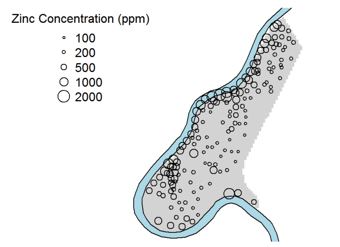
Figure 61. Plot of zinc concentrations in soil near River Meuse, The Netherlands.

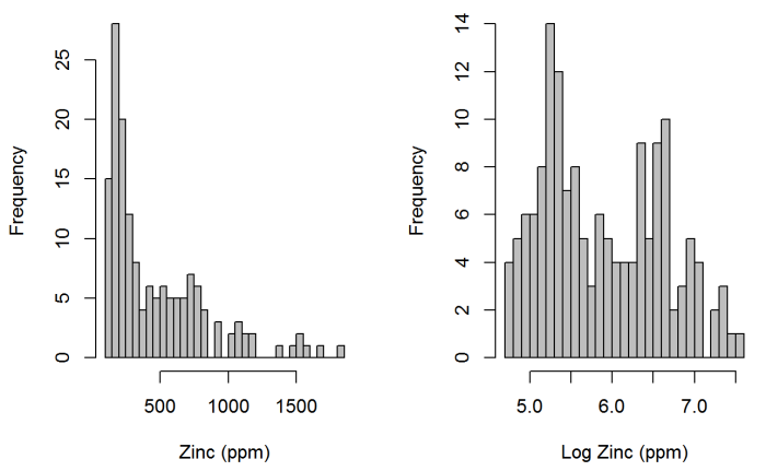
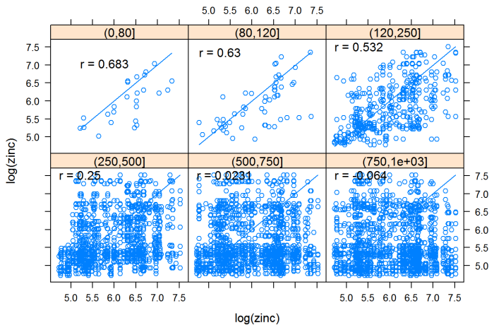
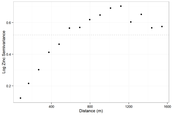
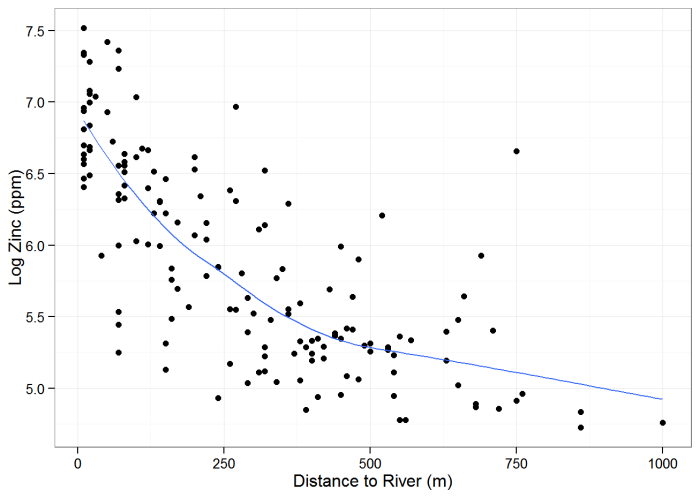
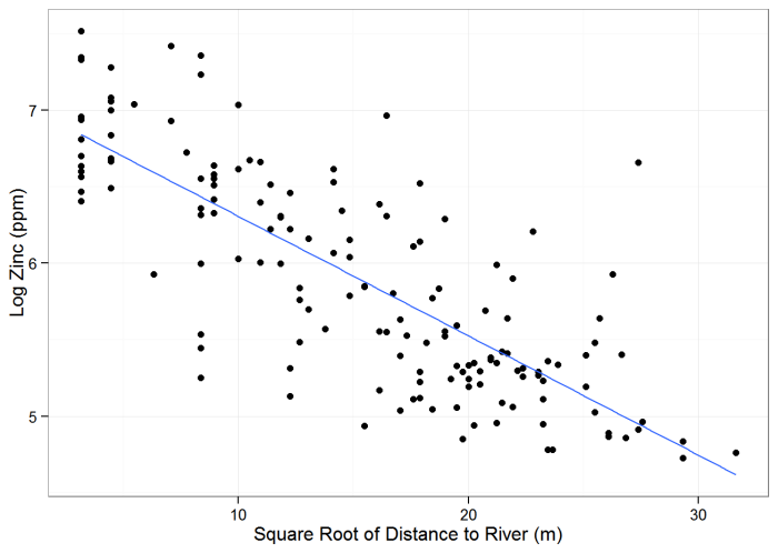
Exploratory Data Analysis – River Meuse

▼Read more

A basic exploratory data analysis is performed using a histogram (Figure 62). The histogram shows the zinc concentrations are highly skewed. Any interpolation method will work better if it transforms the concentrations to make the data more symmetric. A logarithmic (log) transformation is often used to transform concentrations, and so that approach is used here.

gro_fig_62__8_5_cropped

Figure 62. Histograms of zinc concentrations.

The map shows that the zinc concentrations are spatially correlated. This conclusion can be confirmed by looking at the h-scattergram in Figure 63, which shows on a scatter plot all pairs of data points having a specified range of separation distances. The correlation coefficients are also shown on the plots. For example, the correlation between pairs of points less than 80 m apart is 0.683. Up to a separation distance of approximately 500 m, there is still significant spatial correlation between zinc concentrations. This correlation suggests that the spatial coordinates will make reasonable predictor variables in the regression. The variogram shown in Figure 64 is another way to examine spatial correlation. In this case, the variogram confirms that the range of spatial correlation is approximately 500 m. The horizontal dashed line is the variance of the log of zinc concentrations (log zinc). The semivariance reaches the variance at approximately 500 m.

gro_fig_63__8_6_cropped

Figure 63. H-scattergrams.

gro_fig_64__8_7_cropped

Figure 64. Variogram.

The concentrations of zinc are higher near the river. Figure 65 shows that the relationship between log zinc concentrations and distance to the river is nonlinear. By taking the square root of the distance, however, the relationship becomes approximately linear. Figure 66 shows the log zinc concentrations as a function of the square root of the distance.

gro_fig_8_8

Figure 65. Relationship between log zinc concentration and distance to the river.

gro_fig_8_9

Figure 66. Log zinc concentrations as a function of the square root of the distance.

The other available covariates (or predictor variables) for this site are soil type and flood frequency. Three soil types have been identified throughout the area of interest (Figure 67). As shown in Figure 68, the boxplot, type 1 soil is associated with higher zinc concentrations than the other types. An alternative to the box plot is a density plot. The density plot in Figure 69 shows that type 3 soil is associated with a wide range of log zinc concentrations, so this soil type may not contribute much to prediction accuracy. Flood frequency is shown in Figure 70, and the flood frequency class box plot in Figure 71. Flood frequency has also been categorized into three classes, with class 1 (closest to the river) representing the locations that flood most frequently.

gro_fig_8_10

Figure 67. Soil type map.

gro_fig_8_11

Figure 68. Soil type box plots.

gro_fig_8_12

Figure 69. Soil type probability density plot showing the frequency of zinc concentrations for each soil type.

gro_fig_8_13

Figure 70. Flood frequency class 1 (closest to the river) representing the locations that flood most frequently.

gro_fig_8_14

Figure 71. Flood frequency class box plots.

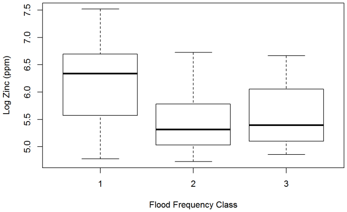
Parametric Regression – River Meuse

▼Read more

A simple parametric linear regression model predicts zinc concentrations from the three predictor variables available: soil type, flood frequency, and distance to the river. The model diagnostic output from the R package mgcv is shown below. The fit is reasonably good, with an R-squared value of 66%, meaning that the model can predict approximately 66% of the variation in the data. The generalized cross validation (GCV) score is 0.163. Comparing this score to the GCV score for an alternative model determines which model is better. Figure 72 includes the diagnostic plots which show that the assumptions of linear regression are approximately satisfied.

Diagnostic Output from the R Package mgcv

##
## Family: Gamma
## Link function: log
##
## Formula:
## zinc ~ soil + sqrt(dist) + ffreq
##
## Parametric coefficients:
## Estimate Std. Error t value Pr(>|t|)
## (Intercept) 7.06916 0.07571 93.376 < 2e-16 ***
## soil2 -0.37666 0.09493 -3.968 0.000112 ***
## soil3 -0.23286 0.14926 -1.560 0.120854
## sqrt(dist) -1.75893 0.20808 -8.453 2.39e-14 ***
## ffreq2 -0.46702 0.08726 -5.352 3.22e-07 ***
## ffreq3 -0.46302 0.10744 -4.310 2.96e-05 ***
## —
## Signif. codes: 0 ‘***’ 0.001 ‘**’ 0.01 ‘*’ 0.05 ‘.’ 0.1 ‘ ‘ 1
##
##
## R-sq.(adj) = 0.658 Deviance explained = 71.7%
## GCV = 0.16301 Scale est. = 0.17469 n = 155

gro_fig_8_15
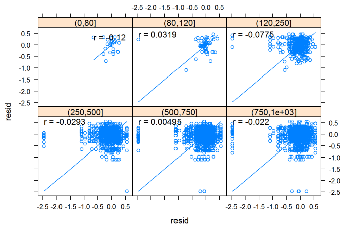
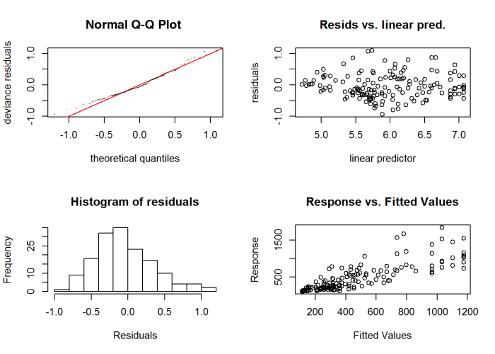
Figure 72. Diagnostic plots.

Nonparametric Regression – River Meuse

▼Read more

Nonparametric regression captures the remaining spatial structure by using a thin-plate regression spline, one of many kinds of splines and kernel methods that could be used. Once the spline is added to the existing model, the R-squared rises to 82%, which is considered good. The GCV score is also significantly lower (0.115). Figure 73 and Figure 74 include the predicted zinc concentrations and associated error.

Diagnostic Output from the R package

##
## Family: Gamma
## Link function: log
##
## Formula:
## zinc ~ s(x, y, bs = “ts”, k = 100) + s(sqrt(dist)) + soil + ffreq
##
## Parametric coefficients:
## Estimate Std. Error t value Pr(>|t|)
## (Intercept) 6.26383 0.05608 111.699 < 2e-16 ***
## soil2 -0.11421 0.10748 -1.063 0.2900
## soil3 -0.30312 0.15727 -1.927 0.0561.
## ffreq2 -0.62153 0.07155 -8.687 1.43e-14 ***
## ffreq3 -0.63759 0.10922 -5.837 4.05e-08 ***
## —
## Signif. codes: 0 ‘***’ 0.001 ‘**’ 0.01 ‘*’ 0.05 ‘.’ 0.1 ‘ ‘ 1
##
## Approximate significance of smooth terms:
## edf Ref.df F p-value
## s(x,y) 17.261 99.000 1.035 2.69e-14 ***
## s(sqrt(dist)) 3.721 4.572 12.387 2.48e-09 ***
## —
## Signif. codes: 0 ‘***’ 0.001 ‘**’ 0.01 ‘*’ 0.05 ‘.’ 0.1 ‘ ‘ 1
##
## R-sq.(adj) = 0.818 Deviance explained = 87.4%
## GCV = 0.11476 Scale est. = 0.082056 n = 155

gro_fig_73__8_16_cropped
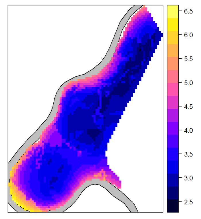
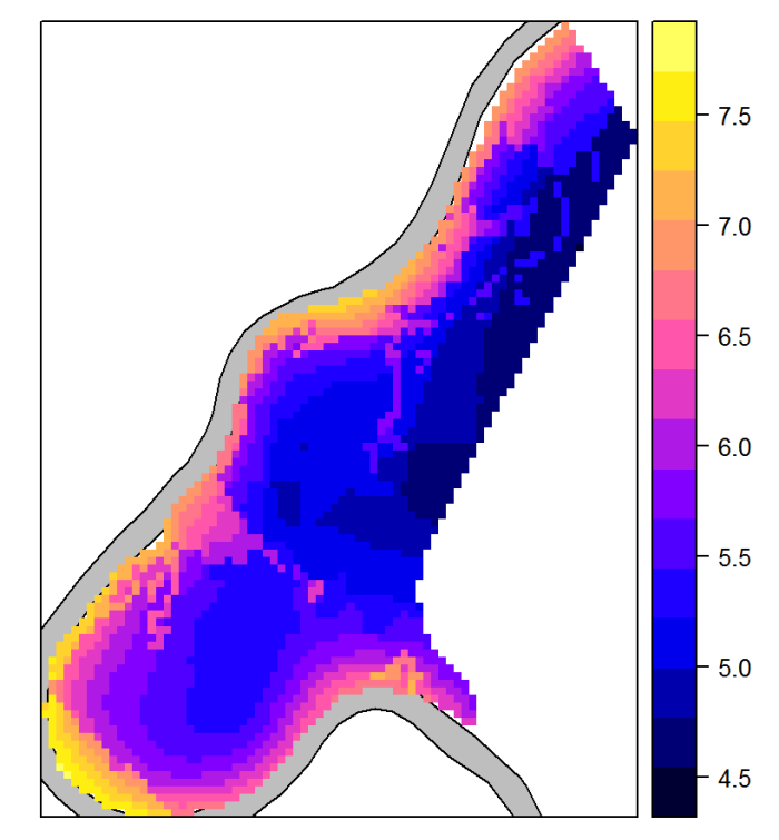
Figure 73. Predicted zinc concentrations.

gro_fig_74__8_17_cropped

Figure 74. Prediction standard error.

If the residuals of the nonparametric model are evaluated using an h-scatterplot (see Figure 75), it becomes clear that they have no remaining spatial correlation. Thus, the model has combined the information from the predictor variables and the spatial correlation.

The model output (predictions and prediction standard error) can now be used for optimization. For example, the output could be used to determine where additional sampling would be most beneficial to reducing uncertainty about the extent of elevated concentrations. The map of predictions shows that the highest concentrations are located along the river shoreline. The map of prediction standard errors shows that within the area of higher concentrations the highest levels of uncertainty are located in the southwest corner of the map at the bend in the river. These areas with the highest uncertainty (highest standard error) should be targeted for additional sampling. Conversely, if resampling of the entire area was planned, the prediction standard errors could be used to indicate areas of low uncertainty where less dense sampling might be appropriate.

gro_fig_75__8_18_cropped

Figure 75. Residuals of the nonparametric model.

image_pdfPrint this page/section


GRO

web document
glossaryGRO Glossary
referencesGRO References
acronymsGRO Acronyms
ITRC
Contact Us
About ITRC
Visit ITRC
social media iconsClick here to visit ITRC on FacebookClick here to visit ITRC on TwitterClick here to visit ITRC on LinkedInITRC on Social Media
about_itrc
Permission is granted to refer to or quote from this publication with the customary acknowledgment of the source (see suggested citation and disclaimer). This web site is owned by ITRC • 1250 H Street, NW • Suite 850 • Washington, DC 20005 • (202) 266-4933 • Email: [email protected] • Terms of Service, Privacy Policy, and Usage Policy ITRC is sponsored by the Environmental Council of the States.