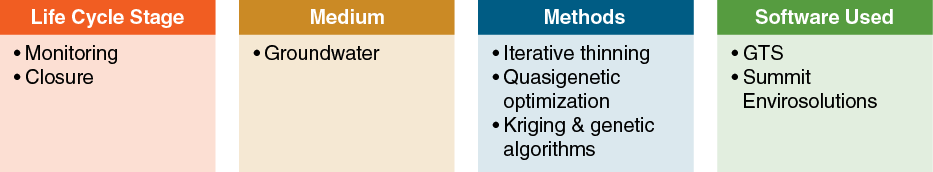
Optimization of Long-Term Monitoring at Former Nebraska Ordnance Plant (GTS; Summit Envirosolutions)
Contact: Kirk Cameron, MacStat Consulting, [email protected]; Phil Hunter AFCEC, [email protected]; Dave Becker, U.S. Army Corps of Engineers, [email protected]
Problem Statement
The former Army Nebraska Ordnance Plant (NOP) occupies approximately 17,250 acres near the town of Mead, Nebraska. During World War II and the Korean Conflict, bombs, shells, and rockets were assembled at the site. The site includes four load lines, as well as the Burning/Proving Grounds, a Bomb Booster Assembly Area, an Air Force Ballistic Missile Division Technical Area, and an Atlas Missile Area.
Wastewater with contaminants from both the load line plant operations and a laundry was discharged into a series of sumps, ditches, and underground pipes. TCE was released from various sources including the Atlas missile site. The site was placed on the USEPA National Priorities List (NPL) of Superfund sites in August 1990 because contamination was identified in groundwater and soils at the site.
GTS was used to evaluate groundwater monitoring data at the NOP site during postclosure long-term monitoring in order to optimize the monitoring network and to demonstrate the usability of the software. In addition, a second evaluation of groundwater monitoring data was made using Summit Envirosolutions software to compare optimization results.
Project Objectives
NOP site groundwater monitoring program objectives were as follows:
- monitor and evaluate potential changes in concentration of contaminants
- provide data to evaluate whether the contaminant plumes are contained by the groundwater extract well network
- evaluate the performance of the site remedy
NOP groundwater monitoring program optimization objectives were as follows:
- determine if there is temporal redundancy in the sampling scheme (are wells being sampled too often?)
- determine if there is spatial redundancy in the monitoring network (are there more monitoring wells than needed?)
- identify areas of site where the monitoring network is inadequate and more sampling locations should be added
- estimate cost savings (if any) that would result if an optimized sampling program were implemented
Site Background
The NOP site is located in the Todd Valley, an abandoned alluvial valley of the ancestral Platte River. The thickness of the unconsolidated material above bedrock in the Todd Valley at the site ranges from approximately 81–157 ft. The unconsolidated material consists of topsoil, loess (predominantly wind-blown silt), sand, and gravel of Pleistocene age. Three aquifers are present at the site: the Omadi Sandstone aquifer, the Todd Valley aquifer, and the Platte River alluvial aquifer.
Monitoring well locations at the site were established based on regional groundwater flow, which is generally towards the south and southeast. The water-bearing portions of the unconsolidated material in the Todd Valley are divided into an upper fine sand unit (12–17 ft thick) and lower sand and gravel unit (17.5–72 ft thick). The upper sand unit is overlain by 4–23 feet of Peoria Loess. Overbank silts and clays ranging from 10–17 ft thick overlie the Platte River alluvial sands and gravels. The water table surface in the Todd Valley slopes toward the south-southeast with depths to groundwater ranging from 6.6 feet to 58.0 ft below ground surface.
Primary contaminants in the identified groundwater plumes include trichloroethene (TCE) and explosive compound hexahydro-1,3,5-trinitro-1,3,5-triazine (RDX). Migration of these contaminant plumes is dictated primarily by the southeastward direction of groundwater flow. Wider-spread groundwater contamination is found in the upper fine sand units than in the sand and gravel units below. Lower contaminant concentrations are generally found in the deepest of the three aquifers.
Four groundwater contamination plumes were identified at the NOP site:
- TCE plume suspected to originate from the Atlas Missile Area, north of the eastern load lines (LL) LL3 and LL4
- TCE plume suspected to originate from LL1
- RDX plumes suspected to originate from LL1 through LL4
Data Set
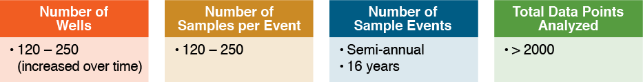
Site-wide sampling at the former NOP began in 1992. The monitoring network has expanded significantly over the years and at the time of the optimization analysis consisted of 257 monitoring wells, plus additional residential and production wells. Sampling had been conducted at various times during characterization and design, but since about 2002 has been generally conducted semiannually. Production and residential wells had, in some cases, been sampled quarterly. The data spanned the time interval of August 1992 to April 2008. Concentrations for seven contaminants were used: TCE, RDX, trinitrotoluene, methylene chloride, dinitrotoluene, trinitrobenzene, 1,2-dichloropropane. Over 2400 specific date/well records were considered in the analysis.
Methods and Results (GTS)
GTS was developed by AFCEC as a publicly available, freeware software application for conducting optimization of long-term groundwater monitoring networks (LTMO). During its development, GTS was tested at a number of Air Force and Department of Defense (DOD) sites, including the NOP site. GTS uses statistical tools and existing groundwater monitoring data to answer two key questions: (1) what is the optimal sampling frequency of monitoring? and (2) what is the optimal number and arrangement of sampling locations in the monitoring network? Unlike some optimization methodologies, GTS does not use fate and transport or other geophysical models of a site. Instead, it bases its optimization recommendations strictly on the statistical properties and patterns evident within the historical sampling data.
All of the statistical optimization analysis was conducted using the stand-alone GTS software application. Cost-benefit analysis of the potential savings associated with an optimized program was done using a separate GTS cost-benefit calculator spreadsheet (Excel). GTS includes tools for data import, data exploration and contaminant ranking, estimating baseline trends and maps, temporal and spatial optimization, and predicting whether new data are consistent with previous trends and plume estimates.
At NOP, GTS was applied separately to all three aquifer zones (shallow, medium, deep), with substantially different levels of spatial redundancy in each zone (termed a 2.5D analysis in GTS), using the two contaminant drivers TCE and RDX. By request of site regulators, 77 of the 250 distinct well locations were protected from optimization, meaning the data from those wells were used to prepare plume maps, but none of those particular locations could be flagged as redundant. Of the unprotected wells, 46% in the deep zone were flagged as redundant, 13% in the medium-depth zone, and 4% in the shallow zone. Figure 91 shows the monitoring wells flagged protected, critical, and redundant in the deep aquifer.
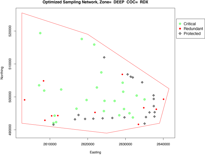
Figure 91. Optimized sampling network for RDX in the Deep Zone.
The monitoring well network was also analyzed to determine whether any new well locations should be added. GTS creates a map across each aquifer zone of the statistical uncertainty associated with all unsampled locations, then preferentially picks locations with high uncertainty and higher nearby contaminant concentrations. The software initially suggested 14 possible new sampling points, but since GTS cannot account for physical obstructions (for example, buildings) or other infeasible locations, only 10 new wells were ultimately recommended.
Iterative thinning was also conducted for all contaminant-well pairs having at least eight distinct sampling events in the data record in order to optimize sampling frequencies. The majority of wells in each aquifer zone were sampled semiannually (2Q) at the time of the demonstration. Iterative thinning suggested that adequate trend reconstruction could be done based on annual (4Q) sampling in two of the three aquifer zones, and every three quarters (3Q) in the remaining shallow zone. Overall, the GTS analysis recommended roughly half of the level of sampling effort that was currently being conducted at existing wells.
The results of the optimization analysis were input into the GTS cost-comparison calculator and are summarized in Table 12. Starting with a baseline of 250 wells and a generally semiannual sampling frequency, and given the typical field sampling, mobilization, and laboratory costs associated with the NOP site, GTS estimated that implementing the optimal sampling plan would result in a net savings of 39% of the annual baseline program cost of $465K.
Table 12. Cost calculator results (Hunter, Cameron, and Stewart 2011)
| NOP Cost Summary | ||
|---|---|---|
|
Baseline Program |
Optimized Program |
|
| Wells Monitored Per Year |
250 |
232 |
| Average Sampling Frequency (per well,per year) |
2.6 |
1.1 |
| Annual Costs | ||
|
Sample Analysis |
$272,650 |
$111,300 |
|
Total Annual Program Cost |
$465,412 |
$284,904 |
|
Potential Annual Cost Savings |
$180,508 |
|
|
Percentage Reduction from Baseline |
38.78% |
|
| Return on Investment (Payback) Analysis | ||
|
Cost of New Well Installation: |
$75,000 |
|
|
Cost of New Well Installation: |
$13,5000 |
|
| Cost of New Well Installation: | $88,500 | |
| Cost of New Well Installation: | 6 months | |
Methods and Results (Summit Envirosolutions)
The Summit Envirosolutions tool was used to optimize the sampling network. After careful examination of data patterns, the project team decided not to attempt to perform a spatiotemporal optimization due to the irregularity and sparseness of the recent data. Various geospatial methods in the Model Builder tool were used to recreate the plume maps, including inverse-distance weighting and various kriging methods (quantile, log-transformed, ordinary). The aquifer was divided into shallow, intermediate, and deep zones, and each was analyzed separately. Quantile kriging provided the best recreation of the likely plume shape. Once the model interpretation technique was chosen and a base representation prepared, a genetic algorithm-based approach was used to explore other smaller monitoring networks and the kriged interpolation of the plume map using the selected wells was compared to the base map. Trade-off curves of error versus cost were prepared. TCE and RDX were linked in various ways in the analysis by limiting the either individual or combined maximum errors for the two contaminants in evaluating the various alternative sampling networks. The sampling plan with the largest acceptable error was chosen.
Five combinations of analyses were performed for each aquifer and are listed in Table 13. Only the results of the analysis of the shallow interval are discussed here, because they are representative of the intermediate and deep zone analyses.
Table 13. Combinations of analyses performed (Harre et al. 2009)
| TCE | RDX | ||
|---|---|---|---|
| A1 | interpolated TCE plume with all sampling data (baseline) | B1 | interpolated RDX plume with all sampling data (baseline) |
| A2 | interpolated TCE plume with combined maximum error of TCE/RDX less than 1.0 | B2 | interpolated RDX plume with combined maximum error of TCE/RDX less than 1.0 |
| A3 | interpolated TCE plume with maximum TCE error less than 0.5 | B3 | interpolated RDX plume with maximum RDX error less than 0.5 |
| A4 | interpolated TCE plume with wells recommended to be removed for the plan of maximum RDX error less than 0.5 | B4 | interpolated RDX plume with wells recommended to be removed for the plan of maximum TCE error less than 0.5 |
| A5 | interpolated TCE plume with common wells recommended to be removed by evaluating each COC independently (separate optimization runs) with maximum error of 0.5 for each COC | B5 | interpolated RDX plume with common wells recommended to be removed by evaluating each COC independently (separate optimization runs) with maximum error of 0.5 for each COC |
Each of the approaches in Table 13 are presented in Figure 92. In each optimization run, the plan along the trade-off curve with maximum acceptable error is selected, as described in Table 13.
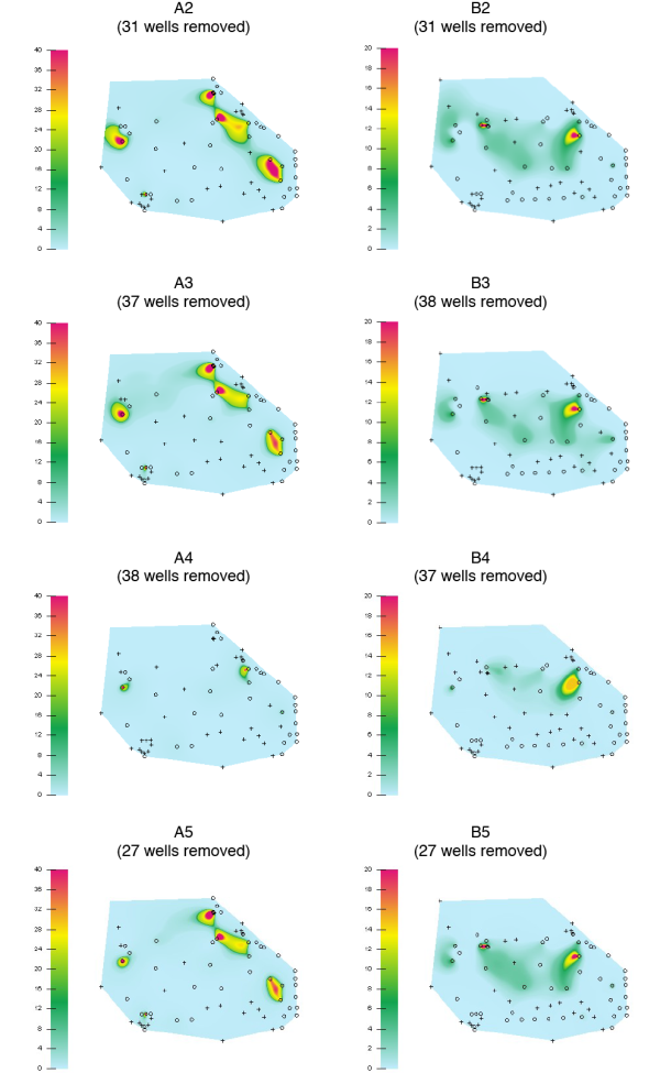 Figure 92. Comparison plume maps. The symbol “+” indicates wells that are recommended to be removed by the Optimizer, while the symbol “O” denotes wells to be kept.
Source: Harre et al. 2009.
A comparison of the plume maps is summarized in Table 14.
Table 14. Comparison of plume map results (Harre et al. 2009)
| Approach | Plume representation | No. of wells removed* | Comment |
|---|---|---|---|
| A2/B2 | Good | 31† | Low cost, good plume interpolation |
| A3/B3 | Good | 37/38* | Low cost, good plume interpolation |
| A4/B4 | Bad | 38/37* | Bad plume interpolation |
| A5/B5 | acceptable | 27 | Conservative, acceptable plume interpolation |
| Note: * 38 wells were recommended to be removed by evaluating RDX only; 37 wells were recommended to be removed by evaluating TCE only. †There are a total of 69 sampled wells in the shallow portion of the aquifer. |
|||
As Harre et al. (2009) report (2009):
The most important result is that A4 and B4, where the wells recommended for removal based on one of the [contaminants] are then removed for the other [contaminant], result in poor plume interpolation. The reason [for this result] is that wells removed for one [contaminant] may be critical for accurate representation of a different [contaminant]. In approaches A2 and B2, where both [contaminants] are analyzed together, the resulting plume representations remain accurate. This process illustrates the benefit of performing the optimization with multiple [contaminants] using the combined error, rather than optimizing them individually. [The team] subsequently used approach A2/B2 (combined maximum error of TCE/RDX) for detailed spatial optimization analysis. Tradeoff curves (sampling cost versus error) for each [contaminant] were generated by the Optimizer tool.
Figure 93 shows, as an example, the resulting cost-error trade-off curve for the shallow aquifer. Figures 94 and 95 show the optimal plans with errors less than 1.0 for the combined TCE and RDX error.
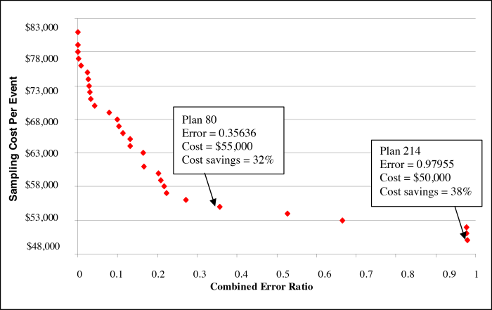
Figure 93. Tradeoff curve for the shallow aquifer
(Number of wells = 81; Number of nonremovable wells = 25).
Source: Harre et al. 2009.
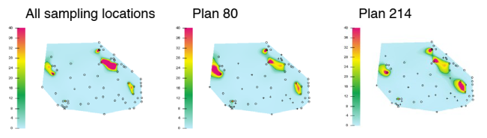 Figure 94. TCE plume map.
Source: Harre et al. 2009.
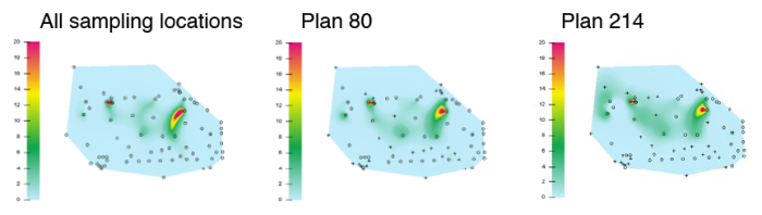 Figure 95. RDX plume map.
Source: Harre et al. 2009.
Harre et al. (2009) further note:
Comparing sampling costs (number of wells multiplied by $1,000 per sample) and errors on the tradeoff curve, and visually inspecting the plume maps for selected plans, Plan 80 and Plan 214 were both considered to be acceptable. [These plans were] both generally similar to the map with all sampling locations for both the higher concentration areas and the lower concentration areas. Of course, [the] site stakeholders will decide if either plan with reduced number of wells is acceptable.
Potential cost reductions were greater than 30%.
Summary of Comparison between GTS and Summit Envirosolutions
The GTS and Summit Envirosolutions monitoring optimization tools were both successful at identifying reduced monitoring programs that would be able to meet the objectives of assessing plume stability as an indication of plume capture/control at a lower cost.
References: Hunter, Cameron, and Stewart 2011; Cameron and Hunter 2000, 2002, 2003, 2004; Cameron 2004; Harre et al. 2009.

